
Today’s guest tutorial comes to you courtesy of X.
In the previous entries of this series, we looked at triangles and circles. This time around, we explore the idea of vectors.
The present article enlarges upon many points made in parts 1 and 2, so interested readers are advised to begin with those.
Vectors (A)
Our study of triangles concluded with a short look at distances. In doing so, we used two representations of points: as objects in their own right, named $ \mathbf{p} $ and $ \mathbf{q} $ in the text, or as bundles of components, $ \vcomps{p_x}{p_y} $ and $ \vcomps{q_x}{q_y} $. These are largely interchangeable, though different situations tend to better suit one or the other. Generally, we favor the whole point approach unless something about the individual components calls for our attention.
While deriving the distance between $ \mathbf{p} $ and $ \mathbf{q} $, the values $dx$ and $dy$ showed up, these being the differences of the points' $x$ and $y$ components, respectively. These can be bundled as well, as $ \vcomps{dx}{dy} $, and given a collective name, say $ \mathbf{v} $.
Now, we subtracted the components of $ \mathbf{p} $ from those of $ \mathbf{q} $. Had we done it the other way around, we would have a slightly different pair: $ \vcomps{-dx}{-dy} $. That is to say, $ \mathbf{v} $ has a built-in sense of direction. This is rather unintuitive with respect to points; conceptually, $ \mathbf{v} $ seems to be another sort of object, namely a vector.
Often these will be written with an arrow up top, as $ \vec{v} $ or $ \vec{\mathbf{v}} $. This article will stick to mere boldface.
Given which components we subtracted from which others, it seems that we could get away with saying $ \mathbf{v} = \mathbf{q} - \mathbf{p}. $ Assuming known rules of arithmetic hold, we could even rearrange this as $ \mathbf{p} + \mathbf{v} = \mathbf{q} $ or $ \mathbf{p} = \mathbf{q} - \mathbf{v}. $
Following the lead of our motivating example, in adding a point and vector, we add the $x$ and $y$ components of each separately, assigning the respective sums to those same components in a new point: $ \vcomps{p_x}{p_y} + \vcomps{v_x}{v_y} = \vcomps{p_x + v_x}{p_y + v_y}. $
Subtraction, which is essentially finding $dx$ and $dy$, proceeds identically, albeit as point minus point: $ \vcomps{q_x}{q_y} - \vcomps{p_x}{p_y} = \vcomps{q_x - p_x}{q_y - p_y}. $
If we slog our way through the vector equations component-wise, everything does indeed check out.
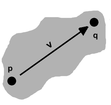
Vectors are often interpreted as paths between two points, as pictured, or displacements from some position. By definition, however, they need only be some object having both a direction and magnitude. (Consider linear velocities and forces, for instance, where physical properties come along for the ride.)


Worth noting is that the definition says nothing about position. Our considerations thus far have looked on them as auxiliary to points, but we can equally well combine vectors with one another. On the left, adding vectors $ \mathbf{v} $ and $ \mathbf{w} $ gives us resultant $ \mathbf{v + w} $. On the right, $ \mathbf{v} + (\mathbf{w - v}) $ sums to $ \mathbf{w} $.
Only certain combinations have been considered in our arithmetic; we did not add points to points, for instance. In fact, a sort of "arithmetic of types" underlies these operations. Imagine our objects carrying around a "type": zero for vectors, one for points. Furthermore, every arithmetic operation, in addition to mixing the objects' components, also determines the type of the result. Some examples:
\begin{align} point + vector & : 1 + 0 = 1 \rightarrow point \\ point - point & : 1 - 1 = 0 \rightarrow vector \\ vector + vector & : 0 + 0 = 0 \rightarrow vector \end{align}
Many combinations give us unknown types, though, such as
\begin{align} point + point & : 1 + 1 = 2 \rightarrow ??? \end{align}
We can rule these possibilities out.
Distinctions aside, points will occasionally be treated as vectors, in what follows. These can be interpreted as the point, say $ \mathbf{p} $, minus the origin $ \vcomps{0}{0} $.
EXERCISES
1. Explain how barycentric coordinates may be added together and still honor our type rules.
Magnitude (B)
In the vectors we have been considering, magnitude means the Euclidean distance from one end (the tail) to the other (the head). This ought to be obvious when, as in the previous section, the vector is shown between two points, being the distance between them. The only novelty here is in considering length apart from a fixed position. We denote this magnitude—from here on out, we will say vector length—by double bars around the name, say as $ \vlen{v} $.
(NOTES: Some of this is redundant in light of the lerp material at the end of triangles)
Knowing how long a vector is, a natural next step is to shorten or extend it. This is achieved easily enough: a vector $s$ times as long has length $ {\mid s \mid}\sqrt{v_x^2 + v_y^2} $. This may be rolled back a bit, to $ \sqrt{s^2}\sqrt{v_x^2 + v_y^2} $ and then $ \sqrt{\left(s v_x \right)^2 + \left(s v_y \right)^2} $. In words, the scale factor simply distributes across components, so $ s\mathbf{v} = \vcomps{sv_x}{sv_y}. $ This vector has the same direction as $ \mathbf{v} $, but is shorter when $ s \lt 1 $ and longer when $ s \gt 1 $.
Note the absolute value of $s$ above. It is perfectly reasonable for $s$ to be negative, so that the vector points away from $ \mathbf{v} $: it then has the opposite sense. The length itself, however, is always positive.
Now, say we have a vector $ \vlen{v} $ units long. What happens if we scale it to be $ 1 \over \vlen{v} $ times as long?
The scaled vector has a length of one, of course! We call these unit vectors, and this particular scaling normalization. It is often much more practical to work with vectors in this form. Such vectors are often written with hats, say as $ \hat{\mathbf{u}} $.
As an immediate application, consider the case where we want a vector to have a specific length, $L$. If the original vector were one unit long, we would just scale it by $L$. In the general case, we need only normalize the vector beforehand and will never know the difference. In fact, we can even pack the two scale factors together as $ L \over \vlen{v} $ and perform everything in one step.
It must be noted that when a vector has a length of zero, or close to it, normalization is nonsensical. In a program this will manifest as a vector with huge or infinite components (and this will propagate through any operations using them). Where such vectors might arise, we should include checks that they have at least some minimum length (or squared length), and only in that event proceed with the code in question.
(IMAGES: 4, 5)
The dot product (C)
Earlier, we alluded to the vector $ \mathbf{w - v} $. From the picture, we see that it completes a triangle begun by vectors $ \mathbf{v} $ and $ \mathbf{w} $. Its length is $ \sqrt{\left(w_x - v_x \right)^2 + \left(w_y - v_y \right)^2} $; expanding the terms inside this root gives us $ w_x^2 - 2v_x w_x + v_x^2 + w_y^2 - 2v_y w_y + v_y^2 $.
Parts of this ought to look familiar. $ v_x^2 + v_y^2 $ is the squared length of $ \mathbf{v} $. Likewise for $ \mathbf{w} $. A bit of rewriting gives us $ \vlen{v}^2 + \vlen{w}^2 - 2(\dotp{v}{w}) $. This has a sum of two squares, almost making it compatible with the $ x^2 + y^2 = z^2 $ format we know from the Pythagorean theorem. When $ \dotp{v}{w} = 0, $ in fact, it will be in exactly that form.
This construction, $ \dotp{v}{w} $, is the so-called dot product, often written as $ \dotvw{v}{w} $.
Before we proceed, consider a vector that is the sum of two vectors, such as $ \mathbf{v} = \mathbf{a} + \mathbf{b} $. In component form, $ \softerdotvw{\vcomps{a_x + b_x}{a_y + b_y}}{w} = \dotp{a}{w} + \dotp{b}{w}. $ The dot product distributes! The same will be found for $ \mathbf{v} = \mathbf{a} - \mathbf{b}. $
We will need a couple other useful properties as we go on, which can be similarly verified: $ \dotvw{v}{w} = \dotvw{w}{v} $ and $ \dotvw{v}{v} = \vlen{v}^2. $
To those familiar with slopes, this ought to seem familiar. When two lines are perpendicular, the slope of one is the negative reciprocal of the other; this is the same phenomenon. (The vector form is robust against horizontal and vertical lines, though, where slopes run aground.)
(NOTES: join)
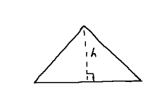
Consider a non-right triangle. As we saw in part 1, any altitude will separate this into two right triangles. The altitude gives these two triangles a common height, $h$.
Now, imagine some vectors incorporated into the mix: one of them, say $ \mathbf{v} $, sits atop the hypotenuse of one of the right triangles, while its companion, $ \mathbf{w} $, overlies the original base. These are just sides, of course, so there is an angle between them.
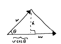
In part 2, we saw how, at any given angle $\theta$ in a circle of radius $r$, we would have a right triangle where $ dx = r\cos\theta $ and $ dy = r\sin\theta. $ We have two of the ingredients: right triangle and angle. Interpreting the hypotenuse, $ \vlen{v} $, as a radius, completes the picture. Reading things back into our triangle, then, it has base $ \vlen{v}\cos\theta $ and height $ \vlen{v}\sin\theta $.
This base uses up part of the full length, $ \vlen{w} $. The other right triangle gets the leftovers: $ \vlen{w} - \vlen{v}\cos\theta $. The Pythagorean theorem glues the remaining bits together: $ (\vlen{w} - \vlen{v}\cos\theta)^2 + h^2 = \vlen{w - v}^2. $
The right-hand side is what was used in the dot product, whereas we can FOIL much on the left. A couple terms cancel as well, and we get $ h^2 - 2\lenvw{v}{w}\cos\theta + \vlen{v}^2\cos^2\theta = \vlen{v}^2 - 2(\dotvw{v}{w}). $ After subtituting $ \vlen{v}\sin\theta $ for the shared height $h$, the left-hand side contains $ \vlen{v}^2(\cos^2\theta + \sin^2\theta) $. As we saw in part 2, the parenthesized part is exactly one. This sets off a short spree of cancellation, culminating in $ \lenvw{v}{w}\cos\theta = \dotvw{v}{w}. $
Typically one last rearrangement follows: $ \cos\theta = {\dotvw{v}{w} \over \lenvw{v}{w}}. $ The dot product associates two vectors with the angle between them. This is extremely important.
The perp operator (D)
When the Pythagorean form is satisfied, we know that we have a right angle. So we immediately find a useful application of the dot product: a result of zero means the two vectors are perpendicular. (A synonym, orthogonal, is quite common as well.)
Now, $ v_x v_y - v_x v_y = 0. $ This would seem almost too obvious to mention, but notice how closely it resembles a dot product.
In fact, it is one, albeit without the nice pairing of $x$ and $y$ labels: $ \vcomps{v_x}{v_y}\cdot\vcomps{-v_y}{v_x} $ and $ \vcomps{v_x}{v_y}\cdot\vcomps{v_y}{-v_x} $ both resolve to the left-hand side.
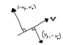
Notice what this is saying. Given a vector $ \mathbf{v} = \vcomps{v_x}{v_y}, $ we have all we need to obtain another vector, $ \mathbf{v^{\perp}} $, perpendicular to it: just swap the components and flip one of their signs. Some sources call this the perp operator.
(NOTES: Something about fixed relative orientation; CW/CCW as per rejection)
(NOTES: Successive application of operator... could bring up in last few sections about intersection)
Projection (E)
The dot product makes no assumptions about its vectors. They may point anywhere, yet it holds.
Consider again vectors $ \mathbf{v} $ and $ \mathbf{w} $ from the last section, and the right triangle arising from them with base $ \vlen{v}\cos\theta $.
As we just discovered, we can extract the cosine (without ever needing to know the angle!) from the dot product. Thus, the base length may also be written as $ {\vlen{v}(\dotvw{v}{w}) \over \lenvw{v}{w}} = {\dotvw{v}{w} \over \vlen{w}}. $
This is the component of $ \mathbf{v} $ in the $ \mathbf{w} $ direction, or $ \mathbf{comp_w v} $, which says how much of $ \mathbf{v} $ can be described by $ \mathbf{w} $. We will run into it again shortly and develop this idea a bit further.
As we have seen a couple times now, it is often useful to use vectors aligned with one of a triangle's side. As far as the base goes, it will have the same direction as $ \mathbf{w} $. Generally, $ \mathbf{w} $ will not be a unit vector, so this calls for the process alluded to earlier: normalize $ \mathbf{w} $, then scale the result to the base length. Taken together, we have a scale factor of $ \dotvw{v}{w} \over \vlen{w}^2 $. It is also not unusual to see this written as $ \dotvw{v}{w} \over \dotvw{w}{w} $, although the two forms are interchangeable.
The vector $ \left(\dotvw{v}{w} \over \dotvw{w}{w} \right)\mathbf{w} $ is known as the projection of $ \mathbf{v} $ onto $ \mathbf{w} $, or $ \mathbf{proj_w v} $. It gives us the vector "below" $ \mathbf{v} $ on $ \mathbf{w} $, its shadow as it were. (TODO: image)
(IMAGE: 9)
The projection coincides with the base of the triangle. Were we to follow the neighboring side upwards, we would get back to $ \mathbf{v} $. We can easily find this vector, the so-called rejection of $ \mathbf{v} $ from $ \mathbf{w}, $ by subtraction, following the examples in earlier images: $ \mathbf{v} - \mathbf{proj_w v} $.
As an aside, while we can go from $ \mathbf{w} $ to $ \mathbf{v} $ via addition, if we instead subtract the rejection from $ \mathbf{w}, $ we end up reflecting $ \mathbf{v} $ across $ \mathbf{w} $: $ \mathbf{v'} = \mathbf{proj_w v} - (\mathbf{v} - \mathbf{proj_w v}), $ or more simply $ \mathbf{v'} = 2 \mathbf{proj_w v} - \mathbf{v}. $ (TODO: image)
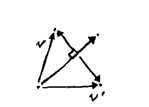
This is a vector perpendicular to $ \mathbf{w} $, along the lines of the perp operator. In that case, however, the right angle is either clockwise or counter- lockwise with respect to $ \mathbf{w} $, depending upon which definition of perp was chosen. The rejection, on the other hand, always points toward $ \mathbf{v} $. We now have the whole triangle expressed in terms of vectors.
(NOTES: Move the clockwise/CCW stuff up into perp)