
Today’s guest tutorial comes to you courtesy of X.
We pick up where our treatment on triangles left off, venturing now into the territory of circles.
Rather than cover old ground, the reader is assumed to be familiar with various concepts already discussed. Those who have not done so are strongly advised to begin with the previous article.
Some points on circles (A)
Now, what is a circle? We all have some intuition, but we are after something of its nature.
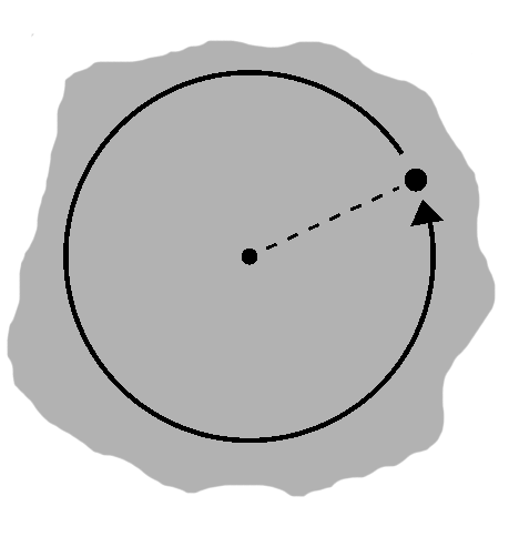
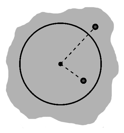
We get some sense of it in a tool used to draw them, the compass. One of its legs, typically with a sharp end, is fixed on a point. Via hinge, the other leg is separated from the first by a certain distance, then locked into place. Along with a bit of pressure to keep it from slipping, we can then turn this second, pencil-equipped leg to draw an arc.
The definition is simply the essence of this mechanism expressed in geometrical language: a circle comprises all points that are a given distance, the so-called radius, from a point called the center. In other words, it is the path traced by one revolution of the compass.
We ended part one by considering lengths of the form $ \sqrt{dx^2 + dy^2} $. The radius, $r$ for short, is just such a length. From the definition, then, $ \sqrt{\left(x - center_x \right)^2 + \left(y - center_y \right)^2} = r. $ This is often written as $ (x - center_x)^2 + (y - center_y)^2 = r^2, $ both sides having been squared. Quite frequently, we need not even deal with the center explicitly, allowing for the simpler $ dx^2 + dy^2 = r^2. $
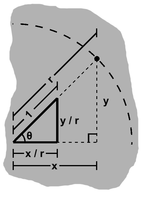
We can divide both sides of the equation by $ r^2 $. Doing so, we get $ \left(\fracalign{dx}{r}{dy} \right)^2 + \left(\frac{dy}{r} \right)^2 = 1. $ This is once again the equation of a circle, this time with a radius of one, known as the unit circle.
(NOTES: Something about arcs belongs here too)
(NOTES: Circle with radius zero, otherwise SDF stuff)
REWRITE REWRITE REWRITE REWRITE REWRITE REWRITE
Say we began with a pin, a pencil, and a string. With the string pinned and held taut, we trace out the path defined for us, sketching as we go. Such a device is known as a compass, and the shape we trace out will be a circle.
The nature of a circle is captured in this device. One of them comprises all points a specific distance from a special point, the center. The center corresponds to the pin and the distance, the radius, the length of the string. The circle is the traced path itself.
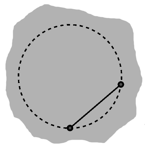
We can make a weaker statement about segments of this circle, say where we started tracing at one part and ended at another, without making the full traversal. We call these arcs.
This definition lets us speak in terms of SDFs, too.
END REWRITE END REWRITE END REWRITE END REWRITE
Cosine and sine (B)
Now, the circle itself is special enough to get its own name. Might there be anything interesting about $ \fracalign{dx}{r}{dy} $ and $ \frac{dy}{r} $?
These are just numbers, of course, so we could arrive at the same values starting from any other radius. In doing so, we would begin with different $dx$ and $dy$ values, too.
Both components have a common scale factor, namely $ \frac{1}{r}. $ If we sketch a few $dx$-$dy$ pairs answering to different values of $r$, it quickly becomes clear that we have similar triangles.
We will see the same phenomenon when we look elsewhere on the circle, although the $ \fracalign{dx}{r}{dy}, \frac{dy}{r} $ pair is unique from place to place.
So, although $dx,$ $dy,$ and $r$ vary, the ratios of $dx$ and $dy$ to $r$ remain fixed, for a given angle opening out from the center. It might be useful if we could work with the angle directly and somehow harness these properties.
Answering this call are two trigonometric functions known as cosine and sine. In terms of an angle called $\theta$, these are defined as $ \cos\theta = \fracalign{dx}{r}{dy} $ and $ \sin\theta = \frac{dy}{r}. $ From the equation of the unit circle we also have the identity (which is to say a relation that is always true, so that two things are "identified" with one another): $ \cos^2\theta + \sin^2\theta = 1. $ These are each of immense importance, foundational to the entire discipline of trigonometry ("the measure of triangles"), to say nothing of mathematics and physics in general.
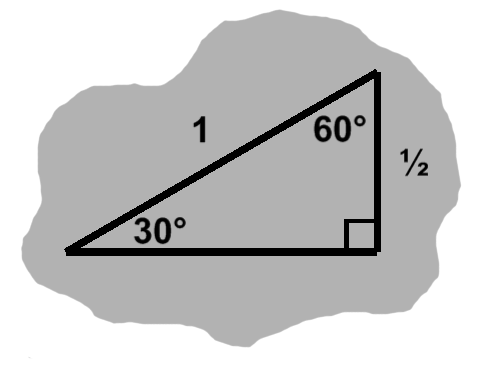
Actually coming up with values for each possible angle would seem like a major hassle, probably requiring many more geometric insights than we have besides. Thankfully, triangles have been objects of fascination since time immemorial; this very antiquity means that other minds have long been doing this painstaking work and tabulating the results, which have steadily improved along the way. These same efforts have also given us solid algorithms to compute these values, so that today in Corona we need only call math.cos or math.sin.
We saw in part one, with the Pythagorean theorem, how we might not have both $x$ and $y,$ but rather one of them together with $z.$ By rearranging the equation, we were able to solve for something other than $z.$ Likewise, we might already have, say, $ \cos\theta. $ If we also knew our radius, we could find $ dx = r\cos\theta. $
(NOTES: Could use a lead-up demonstrating length with similar triangles)
REWRITE REWRITE REWRITE REWRITE REWRITE REWRITE
We saw in part one how to do lengths and also visited the idea of similar triangles. A little demonstration will tie these together.
The triangle comes from how we defined length.
END REWRITE END REWRITE END REWRITE END REWRITE
Adjacent and opposite (C)
Cosine = adjacent, sine = opposite stuff
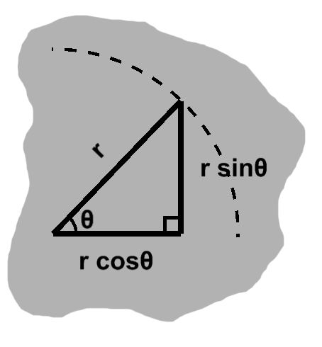
At any given angle $\theta$ in a circle of radius $r,$ we would have a right triangle where $ dx = r\cos\theta $ and $ dy = r\sin\theta. $ We have two of the ingredients: right triangle and angle. Interpreting the hypotenuse, $ \vlen{v}, $ as a radius, completes the picture. Reading things back into our triangle, then, it has base $ \vlen{v}\cos\theta $ and height $ \vlen{v}\sin\theta. $
(NOTES: Earlier idea, i.e. from triangles article, about assuming nice orientation)
(NOTES: Polar coordinates)
So far, we have been treating the triangles as rooted at the right-hand side. As we covered in the first article, often we will begin with an idealized triangle to make our points and then abstract from there.
To this end, rather than the $dx$ and $dy$ we have used thus far, these sides tend to be designated as adjacent and opposite, respectively. These have the same meanings as before, describing their relationship to the angle. This has some interesting outcomes: for instance, the adjacent side might in fact be behind us.
That said, for the moment we will remain with this nice triangle.
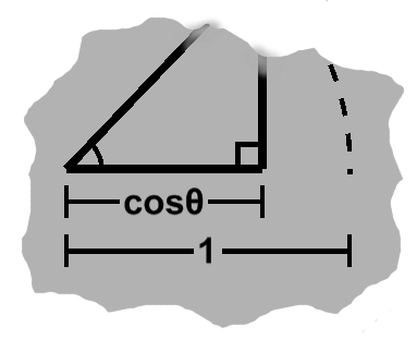
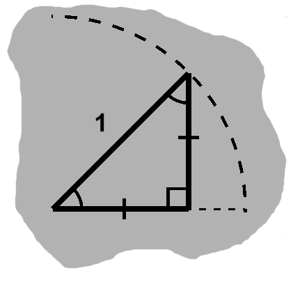
For the majority of angles, the cosine and sine will both be inside of the unit circle. To reach the circle itself, we need to scale these lengths. The unit radius and cosine are in a $1 : \cos\theta$ ratio, of course.
We now have one length. As mentioned earlier, this gives us all we need to produce a similar triangle, since the scaling is uniform. So we can apply it to our cosine-sine triangle.
The other leg of the triangle will have length $\sin\theta\left({1 \over \cos\theta}\right),$ or ${\sin\theta \over \cos\theta}.$ This is typically called the tangent, or $\tan\theta,$ since it only "touches" the circle.
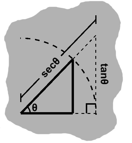
Given an angle and its adjacent side, the tangent lets us calculate the opposite side. This can be convenient, say when the hypotenuse is unknown.
We have the two legs, and can now find the length of the hypotenuse. This is $\sqrt{1 + {\sin^2\theta \over \cos^2\theta}}.$ We can change the inner part to $\sqrt{{\cos^2\theta + \sin^2\theta} \over \cos^2\theta}.$ This becomes the ratio we started with, ${1 \over \cos\theta}.$ This also has a name, the secant, or $\sec\theta,$ since it "cuts" the circle.
Worth noting is that we discovered an identity along the way: $\tan^2\theta + 1 = \sec^2\theta,$ which is occasionally handy.
In the same way, we can find the cotangent and cosecant functions starting from sine.
Historically, several other relationships have been given special names, but have fallen out of favor for whatever reason.
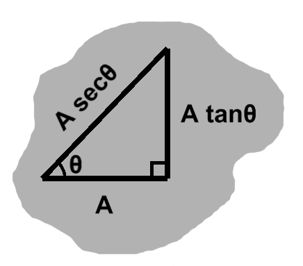
Beyond the motivation, of course, we made little use of the circles. In fact, we can simply pretend one is there, allowing us to generalize these to any situation with a right triangle.
Angle addition (D)
Continuing on the angle theme, recall how adjacent angles summed together.
We begin with the triangle for one of these, as normal.
One for a second rests on top of the original triangle. This is where our opposite-adjacent abstraction comes to the fore, as it no longer aligns with the x-axis.
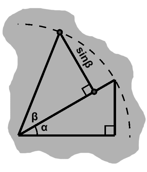
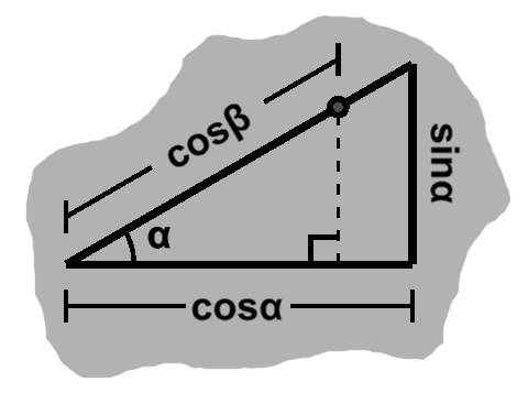
The right angle's corner on the second triangle rests on the hypotenuse of the first triangle, which has length 1 on the unit circle. The distance to this point is $ \cos\beta, $ the length of that side.
We can create a similar triangle from the first triangle, using this length as the common scale factor. Then by scaling the sides of the first triangle, the position of this corner is $ \vcomps{\cos\beta\cos\alpha}{\cos\beta\sin\alpha}. $
Of course, as with our two triangles, we can tease out the triangle for the combined angle, $ \alpha + \beta, $ which will have corner $ \vcomps{\cos(\alpha + \beta)} {\sin(\alpha + \beta)}. $
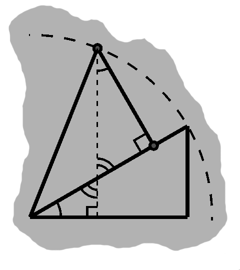
In doing so, we flush out several smaller triangles. On the bottom, we have one similar to the first triangle. As we saw in the previous article, vertical angles are equal, so that carries over to the triangle above. Furthermore, angles sum to 180°, so the angle up top is $\alpha.$
We can further split the above triangle into two smaller right triangles by cutting it horizontally. Up top, we again fill in the missing angle from the sum to 180° (As an aside, note that these both happen to be similar to the first triangle.)
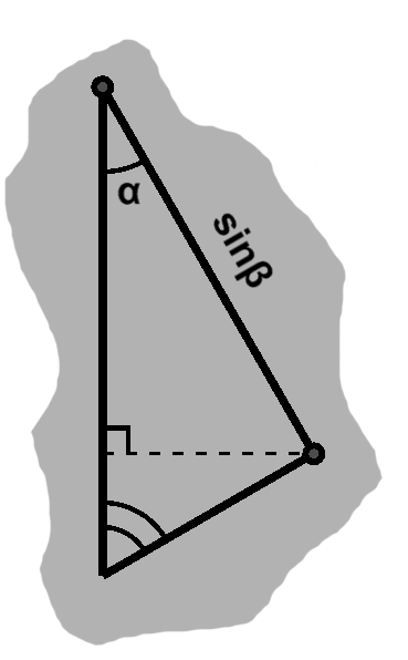
This new top triangle has hypotenuse $ \sin\beta. $ Thus, it has horizontal length of $ \sin\alpha\sin\beta $ and vertical length $ \cos\alpha\sin\beta. $
The corner coincides with that of the second triangle, whereas the upper one is the position of the new angle. So we have
\begin{align} \cos(\alpha + \beta) & = \cos\beta\cos\alpha - \sin\alpha\sin\beta \\ \sin(\alpha + \beta) & = \cos\beta\sin\alpha + \cos\alpha\sin\beta \end{align}
These formulae are invaluable.
Although the circumstances were a bit particular, this actually generalizes to angles in any quadrant or magnitude.
(NOTES: Image to back up last statement?)
(NOTES: Tangent?)
Multiple identities (E)
We can derive some useful results immediately from them, too.
$\sin(\theta + \theta) = \cos\theta\sin\theta + \cos\theta\sin\theta, $ or
\begin{align} \sin 2\theta & = 2\cos\theta\sin\theta \end{align}
In (FIGURE), notice that the right triangle would have area $ \frac{r^2\cos\theta\sin\theta}{2}. $ Given an angle and hypotenuse, then, the area of the triangle is given by $ \frac{r^2}{2}\frac{\sin 2\theta}{2}, $ or $ \frac{r^2\sin 2\theta}{4}. $ The connection between sine and area goes deeper, as we will see in the next article.
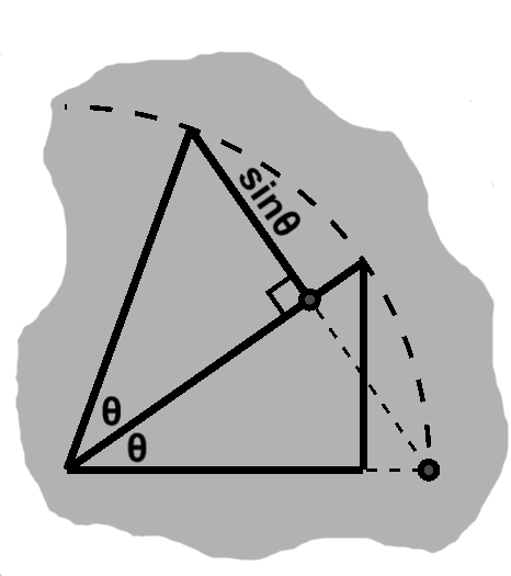
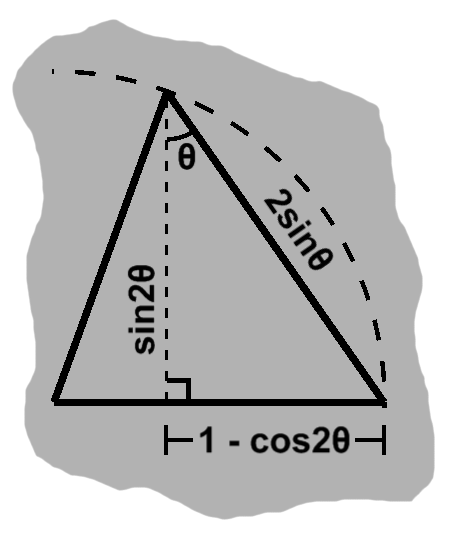
We can see how this looks. Here we have the two triangles stacked as before, forming two halves of an isosceles triangle (TODO: redundant, since this was how we closed article 1). The two opposite sides sum up, so the full triangle has side of $ 2\sin\theta. $
We can draw an altitude down through this triangle, which will have height $ \sin 2\theta. $ In doing so, we will have a case of vertical angles that in turn will bring the angle $ \theta $ up into the other new triangle.
The altitude is its adjacent side, of course, and the hypotenuse $ 2\sin\theta. $ This confirms our identity; in fact, it would have been another way to derive it.
$\cos(\theta + \theta) = \cos\theta\cos\theta - \sin\theta\sin\theta, $ or
\begin{align} \cos 2\theta = \cos^2\theta - \sin^2\theta \end{align}
This last one obviously resembles our previous identity. In fact, we can add 1 to both sides to introduce it: $ 1 + \cos 2\theta = \cos^2\theta + (1 - \sin^2\theta), $ or $ \cos 2\theta = 2\cos^2\theta - 1. $ We can use the identity to go back to sine, too, for a right-hand side of $ 1 - 2\sin^2\theta. $ (We can also get this result from the figure.)
If we plug a half-angle into this last result, we get $ \cos(\frac{\theta}{2} + \frac{\theta}{2}) = 1 - 2\sin^2\frac{\theta}{2}. $
This is already useful, as $ 1 - \cos\theta $ is known to be unstable numerically, so $ 2\sin^2\frac{\theta}{2} $ is often used in its stead.
Furthermore, we can arrange this and solve as $ \sin\frac{\theta}{2} = \pm\sqrt{\frac{1 - \cos\theta}{2}}. $ From the identity, of course, it follows that $ 1 - \cos^2\frac{\theta}{2} = \frac{1 - \cos\theta}{2}. $ After some rearrangement and solving again for a root, we have $ \cos\frac{\theta}{2} = \pm\sqrt{\frac{1 + \cos\theta}{2}}. $ Context will clue us in on which side is appropriate.
(NOTES: Chord length)
(NOTES: Power-lowering)
(NOTES: Probably can make this a legitimate double- and half-angle section, rather than generic identities one)
(NOTES: Tangent)
Settling differences (F)
We would also like to split angles up, which entails differences of angles, $ \alpha - \beta. $
Since this difference will be an angle itself, we can express it in terms of what we just found, with $ \alpha $ as the complete angle and $ \beta $ as the second angle being added.
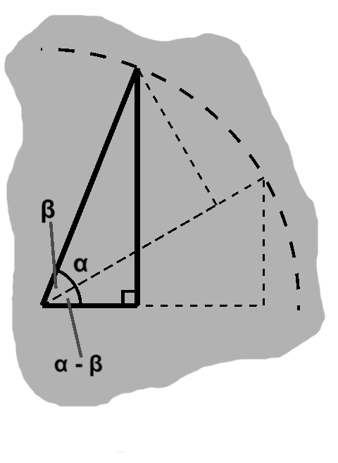
Thus we can plug in $ \alpha = (\alpha - \beta) + \beta $ into our previous equations, giving us
\begin{align} \cos\alpha & = \cos(\alpha - \beta)\cos\beta - \sin(\alpha - \beta)\sin\beta \\ \sin\alpha & = \sin(\alpha - \beta)\cos\beta + \cos(\alpha - \beta)\sin\beta \end{align}
Now, this undoubtedly looks a bit unwieldy, with both cosine and sine in each equation. As with addition, we want them on their own.
We can get some hint of things if we add the two equations together: $ \cos\alpha + \sin\alpha = \cos(\alpha - \beta)(\cos\beta + \sin\beta) + \sin(\alpha - \beta)(\cos\beta - \sin\beta). $
If $ \cos\beta + \sin\beta $ was zero, the cosine would go away and we would have the sine on its own. Likewise, with $ \cos\beta - \sin\beta $ being zero, we isolate the cosine.
Now, these are the terms the equations gave us, so there is not much we can do. However, we can backtrack a bit and start with slightly modified equations.
If the second term were slightly different, $ \cos\beta\sin\beta - \cos\beta\sin\beta, $ the sine would indeed go away. The original $ \sin\beta $ comes from the first equation and $ \cos\beta $ from the second. This suggests scaling the first equation by $ \cos\beta $ and the second by $ \sin\beta. $
In so doing, of course, we must apply the scale factor to all the terms.
After summing the two scaled equations, we have $ \cos\alpha\cos\beta + \sin\alpha\sin\beta = \cos(\alpha - \beta)(\cos^2\beta + \sin^2\beta).$ This simplifies to
\begin{align} \cos(\alpha - \beta) & = \cos\alpha\cos\beta + \sin\alpha\sin\beta \end{align}
The same idea applies to sine, although here we must subtract one equation from the other. This finally boils down to
\begin{align} \sin(\alpha - \beta) & = \sin\alpha\cos\beta - \sin\beta\cos\alpha \end{align}
(NOTES: product-to-sum, sum-to-product identities)
Angles (H)
(NOTES: Can make a point about using angle subtraction to reorient angles, then do addition, etc. Maybe develop from here?)
(NOTES: Needs a bit of repair, and stealing from H, but I think it would be better motivated here)
(NOTES: Furthermore, at 90 degrees and 180 degrees, because circles look the same locally wherever we are--since the distances are the same all around--we can do local analyses as if going from 0 to 90 degrees, then simply apply the appropriate rotations... this gives us the key to take angle addition, and likewise subtraction, past the 90 degree framework in which we derived the equations... I think this would provide a more elegant way to unveil the points about angles that follow, though it will still be a lot of work! Likewise once these points are spelled out the transformation section should have a lot more to refer back to... and perhaps even the computation section.)
We explored angles a bit when we spoke of triangles, much of which carries over to circles.
An angle describes the space between two intersecting sides. Since triangles are closed, we also have the idea of interior angles and sums to 180°.
Moreover, since two of a triangle's points form a line, and the third point is on one side or another, an angle is always less than a straight line.
Circles continue the idea of an opening between sides, though extending it as it continues all around, to the point where the triangle construction falls apart.
Now, on its own this does little for us. A circle is one full revolution, which is not much use as far as angles go.
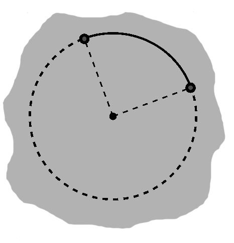
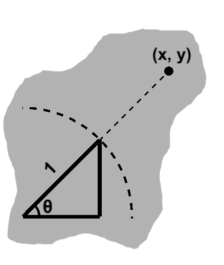
However, angles let us specify points on the circle boundary. In fact, if we rotate the boundary and allow the circle to grow and shrink, we can cover all space, giving us the so-called polar coordinates.
We also now have a useful concept of arc. Starting from the "home" position, the arc goes from there to this position. Generalizing further, with two positions, the arc between them is the longer minus the shorter, which simplifies to their common interval.
These are still points on the circle, so they inherit the distance property.
Now, we run into something if we try to find the arc crossing the "home" position again. We are at a position we have already crossed, but clearly have traveled more distance.
The circle exhibits periodicity. While we can traverse the 360°, we will look as though we had only traversed some. We can decompose the full length. Often we will only care about the remainder.
Further, similar things happen if we go the other way, with negative arcs. We can interpret these as being subtracted from 360° to fix them up. The periodicity will also occur here.
(NOTES: This should be earlier, probably as the second section)
(NOTES: Rough!!!!)
(IMAGES: varieties of angles; triangle)
Transformation (I)
Notice how closely the addition and subtraction formulae match. It almost appears consistent with feeding $ \alpha - \beta $ to the addition formula as $ \alpha + (-\beta). $
To shore up the gap, it must be so that $ \cos(-\beta) = \cos\beta $ and $ \sin(-\beta) = -\sin\beta.$
In fact, this is the case. Recurring to our earlier analysis about angles and definitions of the cosine and sine. At a given angle, we have two possible values of $y$, one on the upper and the other on the lower semicircle, corresponding to the positive and negative angle. On the other hand, $x$ remains the same.
We can account for this by reviewing the original definition of cosine and sine. On the right half, both values have the same $dx,$ but $dy$ differ in sign; likewise on the left. So our guess checks out.
This gives us an easy way to flip a value vertically, given an angle.
What about horizontally?
In this case we will be a certain angular distance from the center, $ 90^{\circ} - \beta. $ But we want to flip, which requires going twice that distance, for $ 180^{\circ} - 2\beta. $ If we add this to our current angle, we get $ 180^{\circ} - \beta. $
We can plug this into our angle difference equations to confirm the result.
Another way we might have gotten this is to figure that we were $\beta$ from the start, so subtract as much from the end.
This is fairly obvious up top, but this result also holds in the bottom half and with negative angles.
We might also want to flip more generally. We can use either of the previous results to do so. If our axis is at $\theta,$ unrotate by that much to bring it in line with the x-axis, do a vertical flip, then rotate back. Alternatively, unrotate by $ \theta - 90^{\circ}, $ perform a horizontal flip, then rotate back.
The first tactic is simple enough. If the axis to flip around makes an angle of $\beta,$ we need to subtract by that to bring all points in the arc into range, so $ \alpha - \beta. $ At this point, negating the angle will do the flip, so $ \beta - \alpha. $ We then need to undo the rotation, so we add back $ \beta, $ giving us a final angle of $ 2\beta - \alpha. $ Note that when the axis is already aligned, with $ \beta = 0, $ we get $ -\alpha, $ as expected.
In the second, $\gamma$ is the difference from the vertical axis. However, we begin as before. We then plug our angle into the horizontal flip formula, for $ 180^{\circ} - \alpha + \gamma, $ then finally add $\gamma$ back. Now, recall that $\gamma$ is only the divergence from the vertical axis, so we have to add 90°. In other words, $ \gamma = \beta - 90^{\circ}. $ Then we have $ 180^{\circ} - \alpha + 2(\beta - 90^{\circ}), $ which reduces to the previous equation.
(TODO: Reflections)
(TODO: Similarity transformation)
Computation (J)
(NOTES: Is it maybe possible to move the sine wave and arccos / sin / tan stuff in here?)
With all of these identities under our belts, along with a few known values, we have what we need to calculate fairly arbitrary cosine and sine results.
First off we can bring angles outside the range back, via the modulus. This simplifies things quite a bit.
Now if our identities hold, we can both start and end at the start angle, under the separate guise of 0° and 360°. Further, we know 90°, 180°, and 270°. We also know some of the intermediate angles, though these would quickly follow from some identity magic.
Our idea is to break a number down by halving it, possibly many times, and adding or subtracting such numbers together. This is exactly what our identities let us do.
So for example (some contrived but demonstrative value).
As we can see, this already works. Historically, many of these values were tabulated for easy lookup (indeed, this was even a common procedure in stock programming, when the trigonometric operations were expensive). This would have been, roughly, the process behind them.
Much has improved, but the ideas at root are the same.
A closer look
(NOTES: NEVER MIND... anyhow, we'll be removing all this)
We ought to do a little unpacking of our formulae.
First up, $ \cos^2\theta + \sin^2\theta = 1. $ Owing to the squares, neither of the left-hand terms will be negative. This being so, it must also be the case that $ \cos^2\theta\le 1 $ and $ \sin^2\theta\le 1. $ Of course, if either term is exactly one, the other will be zero.
Pressing further, this means $ {\mid\cos\theta\mid}\le 1 $ and $ {\mid\sin\theta\mid}\le 1. $
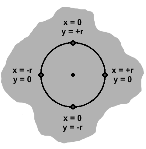
Since $ \cos\theta = \fracalign{dx}{r}{dy} $ and $ \sin\theta = \frac{dy}{r}, $ the minimum and maximum values of cosine and sine occur at $ dx = \pm r $ and $ dy = \pm r, $ respectively.
Without delving too deeply into their properties, it should be evident that cosine and sine are nice smooth functions, since as we take small steps through $\theta$, the corresponding $dx$ and $dy$ values vary only slightly as well.
When $ dx = +r, $ we have $ \cos\theta = 1. $ As mentioned, this must mean that $ \sin\theta = 0 $, corresponding to $ dy = 0. $ By convention, the angle begins counting from here—that is to say, $ \theta = 0^{\circ} $ at $ \vcomps{+r}{0} $—then proceeds counterclockwise.
When $ dx = 0, $ on the other hand, $ \cos\theta = 0. $ In this case, $ \sin\theta = \pm 1, $ and $\theta$ is either 90° or 270°.
With $ dx = -r, $ we end up with $ \cos\theta = -1. $ Again $dy$ and $ \sin\theta $ are both zero, but here $ \theta = 180^{\circ}. $
Sine lends itself to the same sort of analysis. The results, while differing in a few particulars, will more or less rhyme.
We saw that sine could give the same result for different values of $\theta$. At first this might seem a little mysterious, since cosine only takes on one value as we go from right to left. The key is that cosine depends only on $dx$. However, except on the very left or right, there are two points with $dx$ on the unit circle: $ \vcomps{dx}{dy} $ and $ \vcomps{dx}{-dy}: $ one on the top half of the circle and other directly below it, along the bottom.

Cosine is an example of an even function, in that $ \cos\theta = \cos(-\theta). $ We do not find this same symmetry with sine, but rather that $ \sin\theta = -\sin(-\theta). $ The sine is said to be odd.
The takeaway is that cosine is always positive when the angle is small, only going negative once it spills over into the left side of the circle. Sine, meanwhile, is positive so long as the angle remains in the top half of the circle, even when also on the left, and negative once in the bottom half; however, an angle can go directly from zero to negative, so small angles provide no guarantees.
This is quite a lot to take in all at once! These are key details when it comes to developing a geometrical intuition, though, so they are well worth learning.
(NOTES: Carve up, redistribute?)
Round and round we go (K)
Consider something like thread, wound around a spool.
Now, suppose we have enough thread to wrap around once, so the two ends just meet. No stretching allowed!
Obviously, this thread has a length. As this thought experiment demonstrates, this length applies in some sense to the spool, as well, more specifically its circular cross-section. This distance around a circle is called its circumference.
The thread is easily measured, of course. Once unrolled, its length is just the straight-line distance from one end to the other.
Thread was one example, but we could come up with many more, in all shapes and sizes. Soon enough, a relationship seems to emerge: one revolution of the "thread" always shows a circumference just shy of 6.3 times the radius of the "spool".
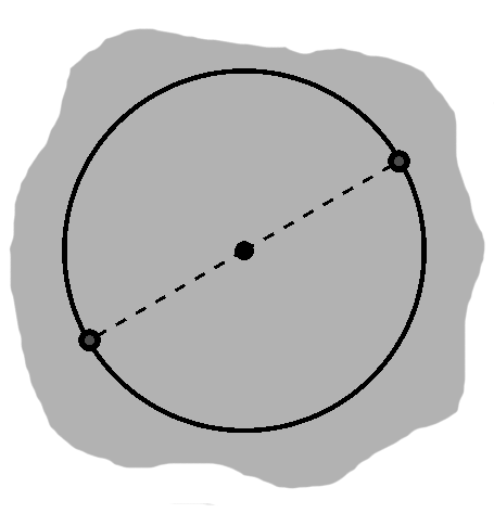
Traditionally, rather than relate the circumference to the radius, which reaches only halfway across the circle—that is, from any given point on the boundary to its center—the diameter is preferred instead. Nothing fancy here; the diameter is simply twice the radius. The ratio of the circumference to the diameter, then, comes out to approximately 3.14159...
This is the famous constant, $ \pi! $
As expressed in mathematical symbols, then, circumference is given by $ 2 \pi r. $
Continuing with the wraparound approach, we can wrap "threads" one-fourth, half, and three-quarters of the original length around our circle. It should come as little surprise that these appear to span the same fraction of the circumference. The facts bear this out for arcs in general, giving us arc lengths of $ (2\pi r)t $, with $ 0 \le t \le 1 $ being the ratio of arc to circumference.
Working with $t$ is a bit awkward, since we then basically already know our arc length. We can streamline this by using angles between 0 and $2\pi$ to traverse the circle. Then arc length is simply $ L = r\theta. $ In the unit circle, for that matter, angle and arc length are one and the same.
Such angles are known as radians. Frequently, in geometry, and almost exclusively in trigonometry, these will be the preferred unit of angular measure. Rather than 90°, 180°, 270°, and 360°, it is quite common to see $ {\pi\over 2}, $ $\pi,$ $ {3\pi\over 2}, $ and $ 2\pi $ in mathematical texts.
Thankfully, the ranges $ [0, 2\pi] $ and $ [0, 360] $ differ only by a constant scale factor. A measurement denominated in degrees can be multiplied by $ \pi \over 180 $ to convert it to radians, while $ 180 \over \pi $ will achieve the reverse. In fact, Lua—and thus Corona—even provides a couple helper functions, so we need not even remember these values: math.deg and math.rad.
local rad = math.rad
local sin = math.sin

function PI ( n )
  -- At the outset, we have three 60-degree triangles, or 3 * (2 * sin(30 degrees)). At each
  -- iteration, we halve all the angles and double the triangle count.
  local count = 2^(n + 1)

  return 3 * count * sin( rad( 60 / count ) )
end

print( PI( 15 ) ) -- on my machine, prints 3.1415926534561...
print( math.pi ) -- ...and 3.1415926535898
This sample is a little circular, as it converts to radians in the process. We can use our earlier half-angle identities, however.
local sqrt = math.sqrt

local function Sin ( steps )
  local cosa = sqrt( 3 ) / 2 -- start with cos(60 degrees)

  for i = 1, steps - 1 do
    cosa = sqrt( (1 + cosa) / 2 ) -- get cos(angle / 2)
  end

  return sqrt( 1 - cosa^2 ) -- sin(angle)
end

function PI2 ( n )
  local steps = n + 1
  local count = 2^steps

  return 3 * count * Sin( steps )
end

print( PI2( 13 ) ) -- prints 3.1415926453212
Unfortunately, numerical precision issues begin to accumulate as more steps are taken. But it demonstrates the principle.
REWRITE REWRITE REWRITE REWRITE REWRITE REWRITE
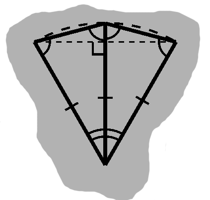
On account of the symmetry of the circle we can deal with just half of that, then later double it.
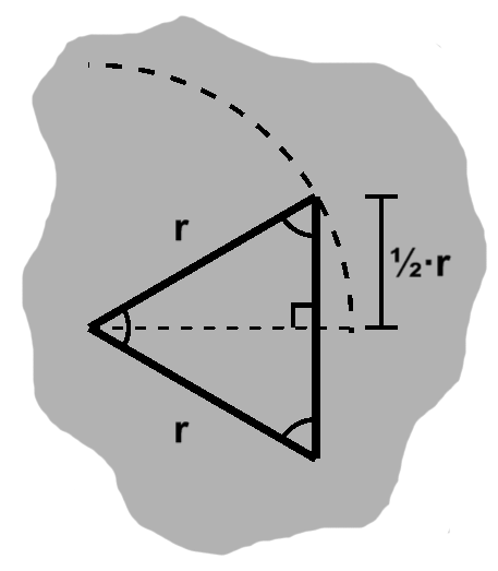
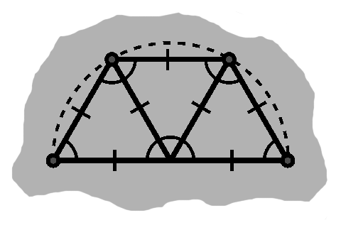
We can then divvy this up into three arcs, which we can approximate by triangles.
In particular, each has 60 degrees. Since two of the sides will be radii, we know the other angles are equal, that is these are equilateral triangles.
Thus the side near the circle boundary also has the radius as length.
So a decent approximation for the boundary is 3 times the radius.
We can divide these in half in turn, which give us our earlier 30-60-90 triangles, which better approximate the circle. (TODO: Not correct, fix)
Gradually, we get nearer and nearer to 3.14159...
END REWRITE END REWRITE END REWRITE END REWRITE
Wheels within wheels (L)
For completeness, we can also look at the area of a circle.
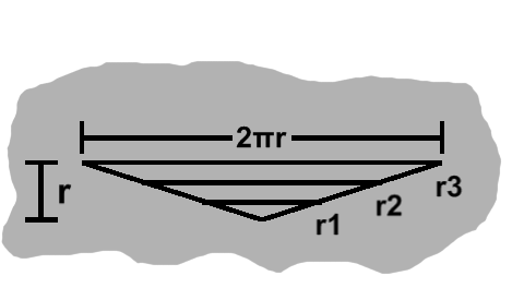
Within a circle, we can highlight any number of concentric circles, which is to say smaller ones that share the same center. In the image on the left, for instance, circles of radius $r_1$ and $r_2$ are nested inside a larger circle of radius $r_3$.
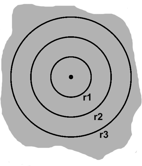
When we consider two consecutive circles, we see that they form a ring. As mentioned, every point on a given circle is equally far from its center, so if we draw a line through two concentric circles, the thickness of this ring will be given by subtracting the lesser radius from the greater one, e.g. $ r_2 - r_1 $.
Now, earlier we saw the connection between circumference and straight line distance. With that in mind, we can draw some conclusions about our pair of circles.
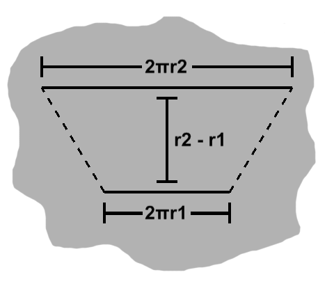
The thickness $ r_2 - r_1 $ was the distance between the two circles, so it makes sense as a height. However, $r_2$ is wider than $r_1$, so we have something that is not quite a rectangle.
This is what is known as a trapezoid, a geometrical object with two parallel sides, usually of different lengths, and a common height.
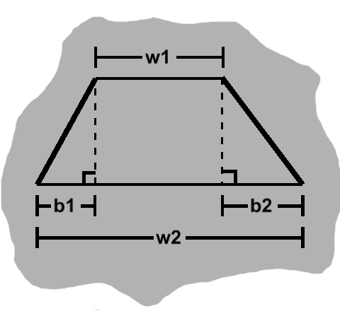
As seen in the image, a trapezoid comprises a rectangle and two right triangles. The longer base has length $ w_2 = w_1 + b_1 + b_2, $ the rectangle has area $ w_1 h $, and the triangles have areas $ b_1 h \over 2 $ and $ b_2 h \over 2 $.
Together, the triangles have area $ (b_1 + b_2)h \over 2 $. We can replace the sum of the triangle bases, using what we know from the length of the longer trapezoid base: $ (w_2 - w_1)h \over 2 $.
Adding the rectangle area to this, our trapezoid has a total area of $ w_1 h + {(w_2 - w_1)h \over 2} $.
Simplifying a little further: $ (w_1 + w_2)h \over 2 $.
Worth noting is that, if the shorter length is zero, this becomes the triangle area formula. (If both sides are equal, on the other hand, we have a rectangle.)
This may be applied to our unrolled rings. The two sides are their respective circumferences, with the thickness as the height. This is $ (2\pi r_1 + 2\pi r_2)(r_2 - r_1) \over 2 $.
This reduces to $ \pi(r_1 + r_2)(r_2 - r_1) $ and in turn $ \pi(r_2^2 - r_1^2) $.
The point about lengths of zero is worth revisiting quickly. Since the side lengths are circumferences in this model, for one to be zero would mean a radius of zero. For consistency, we can call this radius $r_0$. This might seem a little strange, yet it fits snugly into the definition of a circle: all points a distance of zero from the center, the only such candidate being the center itself!
The upshot of this last bit is that the innermost circle can also be streamlined into the ring formulation.
Now, something interesting happens when we start adding these trapezoids together. Here are our three areas lined up:
\begin{align} area_1 & = \pi(r_1^2 - r_0^2) \\ area_2 & = \pi(r_2^2 - r_1^2) \\ area_3 & = \pi(r_3^2 - r_2^2) \end{align}
Comparing subsequent lines, we see $ r_1^2 $, followed by $ -r_1^2 $, and likewise for $r_2$. Thus, after summing all these areas together, what remains is $ \pi r_3^2 $. Since $r_3$ was the outermost radius, we can write the more familiar area formula, $ \pi r^2 $.
Since all these intermediate terms cancel, we could have found the area with more and more circles, even pushing it to the limit where the distance between consecutive circles is infinitesimally small. This might ring a bell to those acquainted with calculus—indeed, the circle area turns out to be the integral of the circumference.
(NOTES: sectors)
(NOTES: Trapezoids slightly more general, e.g. triangle on each side)
The area formula offers us another insight. $ \pi r^2 $ is exactly the area of a triangle with base $ 2\pi r $ and height $r$. And indeed, if we stack all our trapezoids (including the "trapezoid" with one side 0), they coalesce into that very triangle!
Personal space invasion (M)
Recall the definition of the circle: all points a given distance from a common center. Now imagine the situation where we have two circles, not necessarily with the same radius. What would have to be true for them to just touch?
When circles do touch, this means that a point on one circle also belongs to the second circle. We are probably not talking about the trivial case where two circles of equal radius overlap, in which cases this is so for all points. Typically, what we do mean is that the circles interpenetrate—there are two intersections then, in fact, the first when one circle crosses the other going in, the second on the way out. This is true from the point of view of either circle.
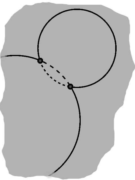
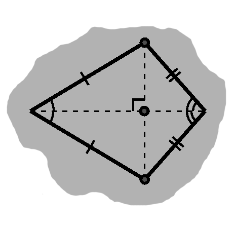
The arcs themselves are interesting, but we can do some other things too. For one, we can draw a line segment between the two intersection points. Furthermore, we can draw line segments from each point to the circle centers, giving us two triangles. Now, those intersection points are, of course, on the circles, so the distance to each respective circle is the radius. In other words, in each triangle, the two lines emerging from the center are equal: this is an isosceles triangle. The angle between them is obviously equal to itself. By side-angle-side, such a triangle is equal to itself. This seems a little silly, but it tells us that we could take the mirror image of the triangle. It follows from this that the other two angles are equal.
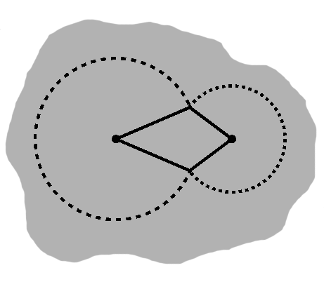
Now, consider what happens when we split this triangle down the middle. We then have side-angle-side again! One side is the radius, we just saw that these angles are equal, and the other side is half of the original length. The angle formed by the dividing line must therefore be the same, which makes these right triangles.
The same thing will happen on both sides. The line between the points of intersection is called a radical line, and as we see it happens to be perpendicular to the line between the circles' centers.
As the circles draw apart, these "in and out" arcs shrink. In other words, their arc lengths diminish, though obviously the circles (to which the arcs belong) are not changing size. Rather, the arc angles are narrowing. When they hit zero, the arcs "enter" and "leave" at the same point. Naturally, the triangles collapse as well, and thus so does the radical line, in fact to this point.
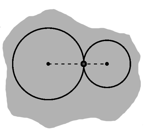
Indeed, this happens to be the point where the circles "just touch". The distance between the centers when this occurs is exactly the sum of the circles' radii: $ \sqrt{(center_{1,x} - center_{2,x})^2 + (center_{1,y} - center_{2,y})^2} = r_1 + r_2. $ (If we will not directly use this distance, but need only compare against it, we may square both sides.)
Now, when the circles were mashed up against one another, this distance was somewhat less. Going the other way, we know when they exceed this distance, the circles are separated and do not touch.
It is worth considering the first case a little more. In particular, when one circle is smaller than the other, it might actually be completely inside the other, without touching its boundary.
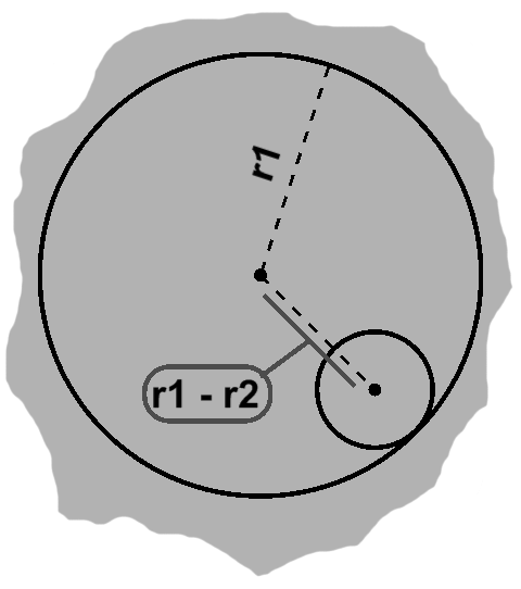
As we saw, we know that it is one or the other when the distance between centers is less than the sum of the radii. That distance is key. We already know how far the smaller circle is from the center, so in a sense we have "used up" that much radius, and there is some amount left. If the smaller circle's radius is not enough to make up the difference, it is completely contained. Otherwise, it touches the boundary.
(NOTES: Intersecting chord midpoints)
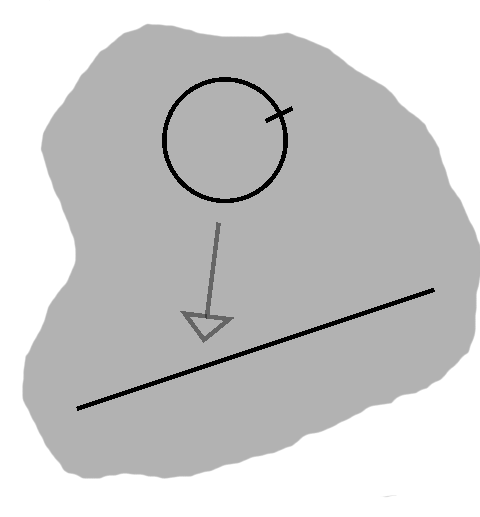
Tangent lines (N)
To get back to points on the circle, for any angle we can of course just find the cosine and sine.
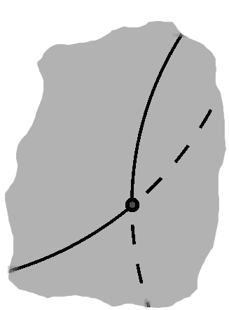
By construction, this is the difference between that point and the center. If we follow the same direction one unit out, we would also have a direction pointing away from the circle, a so-called surface normal.
Now, locally, this direction would be pointing straight up from the circle. If we went straight to the left or right in either direction, we would miss any more of the edge: since points are a radius away, and they have to spend some of that in the curve itself, the space will be empty there.
To go straight left and right implies going 90° away from straight up.
Since the normal's equation is that of the position, we can find one of these candidates by taking the respective measurements: $ x = \cos(\theta + 90^{\circ}) $ and $ y = \sin(\theta + 90^{\circ}). $ We find that $ \cos(\theta + 90^{\circ}) = -\sin\theta $ and $\sin(\theta + 90^{\circ}) = \cos\theta. $
These are useful identities in their own right (as are the variants where we subtract 90°, which will have signs flipped).
These components describe a tangent line, which only touches the circle at this point. (Although the reasons behind the name are the same and they sometimes arise in the same situation, this is different from the trigonometric function described above.)
Together with the normal, these two describe a sort of local coordinate frame above the circle. The next article will explore this idea in more depth.
(NOTES: Can use to "swim" along the surface when combined with re-projection, as in boids)
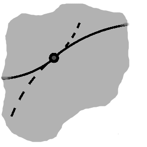
One example of how to apply this is to string circular arcs together nicely. Given two arcs, we can of course just line up one point from each. This can be a bit jarring, though.
If the tangents are pointing in the same (or opposite) directions, however, we have a perfect fit. This is the distinction between C0 and C1 continuity.
Certain functions lend themselves to nice approximations via circular blending curves, so this is a useful part of our toolkit.
In fact, curves assume this behavior locally. In addition to the tangent, the notion of curvature asks what the circle looks like locally, namely its radius.
We can also interpret a segment under this idea. One endpoint is taken as the center, while the offset of the second is converted to polar form. We then take its tangent. This will apply with any length.
A line is its own tangent. Naturally we might suspect it has no curvature. This would comport with it being an infinitely wide circle.
Making waves (O)
We have been treating cosine and sine as means of locating points on the circle, but it can be interesting to consider them in the context of coordinates.
This is fairly straightforward in terms of $y.$ From 0 to $\pi,$ we have $y$ matching the upper semicircle. From there to $2\pi,$ it matches the lower one. We can plot this by stitching the two halves together, as pictured.
(NOTES: image)
This is slightly awkward. The bottom axis of the graph has a certain split definition to accommodate the turnaround, with $x$ changing in different directions. Plotting $x$ would proceed similarly, but we must take the right and left semicircles instead, performing a right angle rotation along the way. In that case, it would be in terms of $y.$
Rather than use $x$ and $y$ as the inputs, the angle would be more natural. This streamlines the input, allowing as well for it to extend indefinitely in either direction, taking in the periodic nature of the functions.
In this case, our graph switches from $ y = \sqrt{1 - x^2} $ to $ y = \sin\theta, $ which changes the shape slightly, giving us a sine wave.
(NOTES: Various properties, use cases)
(NOTES: Other functions)
Getting an angle on things (P)
It was mentioned above that something like $ \cos\theta = {dx \over r} $ could be rearranged, say to find $dx$. This is all well and good, but what if our goal is to recover $\theta$?
The inverse trigonometric functions answer this need. In particular, inverse cosine and sine—available in Corona as math.acos and math.asin, respectively—when given some value between -1 and 1, will return an angle that would have produced that value via the original function. With the example in the previous paragraph, we can extract an angle like so: $ \theta = \cos^{-1}{dx \over r}. $ The $ \cos^{-1} $ and $ \sin^{-1} $ style is often used to denote "inverse", though we will sometimes see arccos and arcsin used as well. The latter form follows upon the insight above that angles and arc lengths are equivalenton the unit circle: "arccos" translates to "the arc length leading to this value of cosine"; likewise for "arcsin".
We noted above that various angles, in fact infinitely many, would produce the same value when fed to cosine and sine. This obviously presents a problem when it comes time to invert! To address this, some canonical range, generally understood to be the best all-around fit, is assigned to each function. In the case of inverse cosine, this is $ [0, \pi] $; for inverse sine, it is $ [-{\pi \over 2}, +{\pi \over 2}] $.
Often enough, these ranges will suit us fine. Otherwise, we will need to rely on additional context to fix the result. If we knew the angle was in the lower half of the circle, for instance, the inverse cosine would need to be corrected to be its reflection instead. Obviously, the more automatic this was, the better.
(NOTES: Identities, another image for that)
(NOTES: chord formulas -> angle)
(IMAGE: 12)
REWRITE REWRITE REWRITE REWRITE REWRITE REWRITE
END REWRITE END REWRITE END REWRITE END REWRITE
Off on a tangent
Now for a little digression.
Another trigonometric function is the tangent, an admixture of the two we have worked with up to this point: $ \tan\theta = {\sin\theta\over\cos\theta}. $
Now, we know that cosine goes to zero at angles like $ -{\pi\over 2} $ and $ \pi\over 2 $, so not only is the tangent undefined there, but it will take on values much larger than one as it draws close. In between, on the other hand, it achieves something of a compromise between cosine and sine.
As with cosine and sine, there is an inverse tangent (see math.atan). Tangent is no exception when it comes to ambiguity, so it too must be constrained. The angles we mentioned as troublesome for our cosine denominator also bound the range of inverse sine; naturally enough, inverse tangent's range is $ (-{\pi \over 2}, +{\pi \over 2}) $. Note the parentheses, rather than brackets: it will not actually give back $ -{\pi \over 2 } $ or $ \pi \over 2 $, since the tangent breaks down there.
In practice, the inverse tangent is not often all that useful. The zero denominators are a hassle. The cosine gets shoehorned into sine's territory. Cosine or sine might be negative, but after division we have only one number, so the details get lost, together with what they might tell us about the angle: when the tangent we wish to solve is negative, we cannot tell whether this came from cosine or sine; when positive, were both cosine and sine themselves positive, or did two negatives cancel out?
The solution, of course, is to do some analysis on $ \cos\theta $ and $ \sin\theta $ beforehand, then use our findings to fix up the results. If $ \cos\theta = 0, $ we know that $ \sin\theta = \pm 1. $ Then, depending on the sign, we have either $ \theta = {\pi \over 2} $ or $ \theta = -{\pi \over 2}. $ Similarly, in the other situations, we can consult the signs to apply the proper corrections.
This is such a common need that a two-argument inverse tangent has become a staple of programming languages. Lua is no exception, offering us math.atan2. These go further and recognize that requiring the inputs to be bonafide cosine and sine values is too limiting—in the real world, for instance, it might be hard to ensure that both perfectly satisfy a common $\theta$. Rather, as long as both are not zero, they accept $x$ and $y$ arguments and do the heavy lifting behind the scenes, inferring the common radius and then $\theta$.
(NOTES: Carve up, redistribute)
REWRITE REWRITE REWRITE REWRITE REWRITE REWRITE
END REWRITE END REWRITE END REWRITE END REWRITE
Summary
Thus far, our investigations have covered triangles and circles. We have examined many of their properties, such as angles, lengths, and areas, and various facts that follow from them.
The next article will bring vectors into the fold. We will explore new ground, of course, but also build on our many discoveries thus far.