
Today’s guest tutorial comes to you courtesy of X.
We pick up where our treatment on triangles left off, venturing now into the territory of circles.
Rather than cover old ground, the reader is assumed to be familiar with various concepts already discussed. Those who have not done so are strongly advised to begin with the previous article.
Some points on circles (A)
Say we had a pencil, plus a sheet of paper held in place by a pin. The pencil and pin are tied together with a piece of string.
We move the pencil away from the pin until the string is taut, place it on the paper, and start to move, maintaining this same distance. Eventually we arrive back where we started.
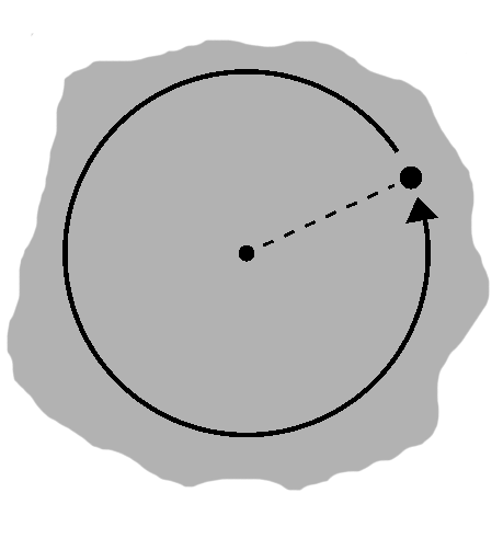
This describes a compass. One full revolution captures mechanically the essence of a circle: all points the same distance away from a central point. In our example, this distance, called the radius, is given by the length of the string, whereas the center corresponds to the pin; the circle is the traced path itself.
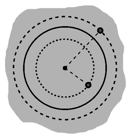
In terms of figure A-1, the dashed segment can be thought of as the string and the smaller dot as the pin. The larger dot represents the pencil somewhere along its path. (The radius terminology is also used for the segment itself, which "radiates" out from the center.)
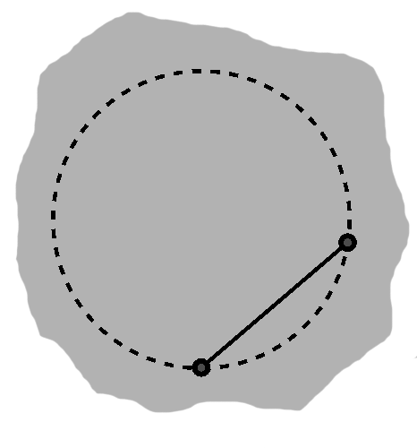
We may draw a line segment between any two points on a circle, as for instance in A-2. Such a segment is known as a chord.
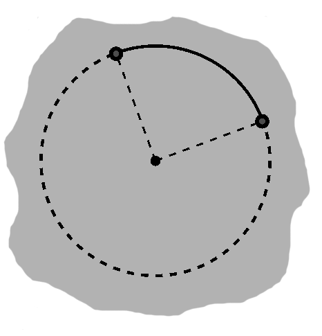
We might instead concentrate on the portion of the circle itself lying between two points. A "circular segment" of this sort, such as the solid curve in A-3, is called an arc. We will always have two arcs, in fact: the dashed curve in that same figure is one as well. Often we only need the shorter of the two.
Figure A-3 highlights a couple of segments emerging from the center. The angle between them is called a central angle.
When we combine a pair of segments like this with one of its associated arcs, they end up enclosing a region inside the circle, or sector. In A-3, using the solid arc etches out a pie slice-shaped sector, while its dashed counterpart gives us something resembling a certain pellet-munching icon of gaming.
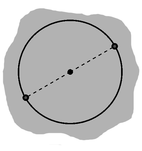
A chord that passes through the center is somewhat notable, since this means its length is twice the radius. Naturally, it has a name meaning "double length": diameter. The points on the circle are said to be antipodal: "feet opposite", like people on the other side of the earth.
A mathematical circle is more restrictive than the colloquial notion most of us have, which is probably something like Corona circles. According to the strict definition, it is only the curve itself, some distance from the center, but not the interior points. In A-5, for instance, neither of the gray points is in the circle, even the one inside. (In geometric language, the circle plus its interior is a disk.)
The two gray points are "some distance" from the same center, of course, so we can say they lie on other concentric circles. The interior point in A-5 will have a smaller radius, the exterior a larger one.
When our radius is $0,$ "all" points are again that far from the center: however, this is nothing but the center itself! This degenerate case is not terribly interesting, though it occasionally arises as a corner case when dealing with lengths. Our analysis will by and large assume "nice" circles.
Cosine and sine (B)
In the last article we considered lengths of the form $\sqrt{dx^2 + dy^2}.$
A radius, $r$ for short, is just such a length. Given a center $\mathbf{c} = (c_x, c_y),$ we have $dx = x - c_x$ and $dy = y - c_y,$ where $x$ and $y$ take on different values as we travel around the circle. Since lengths are never negative, we can safely square this: \begin{align} (x - c_x)^2 + (y - c_y)^2 = r^2 \end{align} This is one of the common forms for circles. As mentioned above, we are going to be focusing on proper circles, with $r > 0.$ This means we can divide by $r^2,$ giving us: \begin{align} \left(dx \over r\right)^2 + \left(dy \over r\right)^2 = 1 \end{align} This describes a circle with radius $1,$ the so-called unit circle.
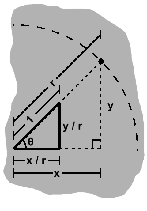
As we also saw in the previous article, scaling is a matter of similar triangles. Angles remain intact despite changes in our radius. Since $\fracalign{dx}{r}{dy}$ and $\frac{dy}{r}$ always divide out the radius, these values are similarly robust. They always describe the width and height, respectively, of a right triangle with one corner on the unit circle and another at its center, as in figure B-1.
The upshot being, the sides of this right triangle only change when the central angle does. Given an angle called $\theta,$ we may therefore express such lengths in terms of it: \begin{align} \cos\theta & = \frac{dx}{r} \\ \sin\theta & = \frac{dy}{r} \end{align} These are the cosine and sine, two trigonometric functions with immense importance in geometry, but also mathematics more generally. Many of our upcoming results will be expressed in terms of these functions, but it is worth keeping in mind that they arise from simple ratios.
We can plug these right back into the unit circle equation above: \begin{align} \cos^2\theta + \sin^2\theta = 1 \end{align} This expression has a tendency to show up again and again, despite its apparent simplicity. It is the first example of an identity, a relationship that is always true and "identifies" two things, allowing us to perform useful substitutions. The discipline of trigonometry, the "measurement of triangles", consists in building up a collection of such identities and putting them into practice.
(NOTES:Comment about notation, i.e. parentheses and powers?)
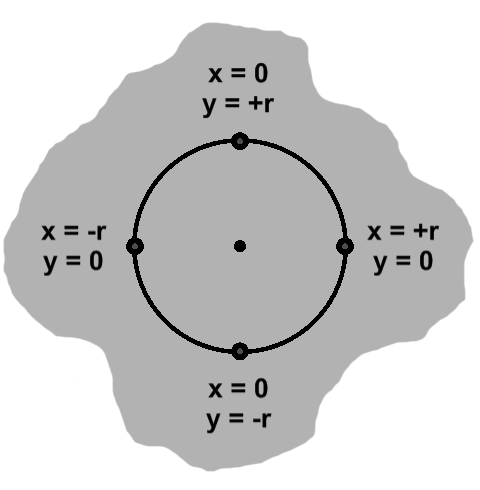
We can identify some values right off. For instance, when $dx = 0, dy = \pm r,$ and likewise when the roles are reversed. This gives us the points at 0°, 90°, 180°, and 270°, as depicted in B-3. Notice that unlike triangles, circles are not limited to 180°.
The arcs formed by consecutive pairs of these points are called quadrant, since they divide the circle into four parts. The range from 0° to 90°, which will be our focus for some time, is the first quadrant.
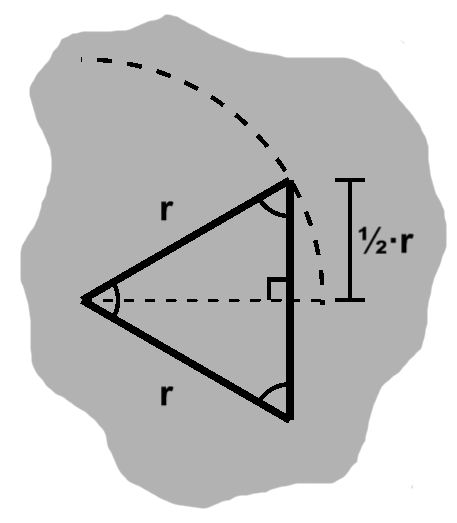
Earlier we saw that in an equilateral triangle, all sides are equal, as well as angles. The triangle postulate tells us these angles must each measure 60°.
We can situate such a triangle so that the x-axis bisects one of its angles, as in B-3. In doing so, we also cut the opposite side in half.
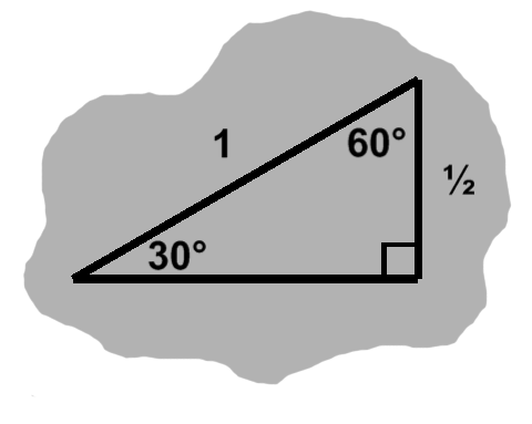
On the unit circle, the upper half takes the form of B-4. Thus: \begin{align} \sin 30^{\circ} = \frac{1}{2} \end{align} This demonstrates the benefits of working on the unit circle: $r = 1,$ so $\sin\theta = dy$ (and $\cos\theta = dx,$ of course). Aside from convenience, this also confers generality on our results; we need only scale the circle and any associated triangles to accommodate the case at hand.
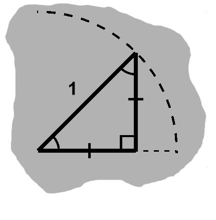
From our shiny new identity: \begin{align} \cos 30^{\circ} & = \sqrt{1 - \sin^2 30^{\circ}} \\ & = \sqrt{1 - \left(\frac{1}{2}\right)^2} \\ & = \frac{\sqrt{3}}{2} \end{align} We can also put a right-angled isosceles triangle down, with one of its sides along the x-axis and a corner on the unit circle, as in figure B-5. The equal angles measure 45°; from the sides, we know that $dx^2 + dx^2 = 1.$ Thus
Filling in the rest of the circle is rather more involved. We will uncover many of the techniques that make doing so possible as the series unfolds.
Thankfully, most of the hard work has already been done here. Not only do we have massive tables of precalculated results, but also solid algorithms to compute cosine and sine directly, so that today in Corona we can simply call math.cos or math.sin.
Polar coordinates (C)
It was mentioned above, in connection with the gray points in A-5, that these were found on other circles sharing the same center but differing in their radius.
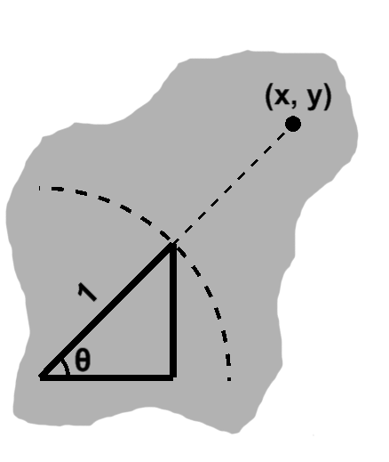
In fact, this describes any point with respect to some circle. In figure C-1, we have a point at $(x, y),$ along with a unit circle. Assuming this circle's center is at the origin, the point will be on a concentric circle with radius \begin{align} r = \sqrt{x^2 + y^2} \end{align} The central angle in this figure, $\theta,$ measures the arc from the x-axis to the line from the center to $(x, y).$
Since we can pick any distance from the center, the corresponding circle contains all points that far away, and we can visit all such points on the circle, it follows that any $(x, y)$ can also be specified as another pair: $(r, \theta)$. These are the polar coordinates.
When the center (the pole, in this context) is at the origin, $x = dx$ and $y = dy.$ We can plug these back into our earlier formulae and rearrange:
On this last bit, note that all angles snap to $x = y = 0$ when our radius is $0.$ This makes rectangular-to-polar conversion ambiguous there: any angle works, but some choices might not play well with typical results.
As an example, say we adopt a policy of always choosing $\theta = 0^{\circ}.$ If we want to travel between concentric circles, we should be okay: $(r + dr, \theta)$ to $(r, \theta)$ is nice and smooth. At the center, things get hairy. From $(dr, 0^{\circ})$ down to $(0, 0^{\circ}),$ all is well, but coming from $(r, 180^{\circ})$ we would spiral in! Interesting at first, but it sticks out like a sore thumb.
Situations like these are left mathematically undefined; the right answer, when there is one, depends on external context.
The pole might be at $(p_x, p_y),$ rather than the origin. In that case, following the ideas above: \begin{align} r & = \sqrt{dx^2 + dy^2} \\ x & = p_x + r\cos\theta \\ y & = p_y + r\sin\theta \end{align}
(NOTES: This is probably stronger if we get the pole stuff out of the way then specialize to the origin)
Tangent and secant (C)
Throughout most of the first quadrant, the cosine and sine will give us a right triangle inside the circle, like we saw in C-2. The only exceptions are found at 0° (cosine $1,$ sine $0$) and 90° (cosine $0,$ sine $1$), which collapse into line segments.
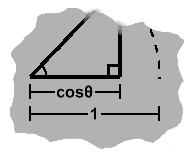
Figure C-3 zooms in on the $dx$ side of such a triangle. The circle's radius is in a $1 : \cos\theta$ ratio with this side.
(NOTES: Should C-4 have 1 at the bottom?)
Applying the scaling factor $\frac{1}{\cos\theta}$ gives us a similar triangle with $dx = r.$ This is depicted with dashed segments in C-4.
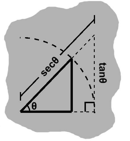
On the unit circle, the $dy$ side of this new triangle has length $\sin\theta\left({1 \over \cos\theta}\right).$ This side only "touches" the circle, so the function for its length is given the name tangent: \begin{align} \tan\theta = \frac{\sin\theta}{\cos\theta} \end{align} In the same way, the scaled hypotenuse has length $1\left({1 \over \cos\theta}\right).$ Since this side "cuts" the circle, the function is called the secant: \begin{align} \sec\theta = \frac{1}{\cos\theta} \end{align}
The Pythagorean theorem then gives us another useful identity:
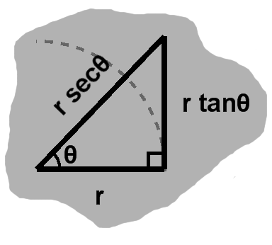
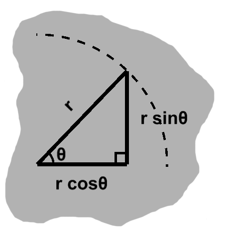
Figure C-5 emphasizes some important relationships that arise when we have a circle of radius $r,$ rather than strictly the unit circle. Given an angle, we can calculate $dy$ or the hypotenuse directly from $dx,$ scaling it it by the tangent or secant of the angle, respectively. This will prove quite useful!
We can also find the so-called cotangent and cosecant functions by applying the above steps to $dy$ and sine. For the most part, these have analogous properties. Historically, various other side-angle relationships have also received special attention as well, but for one reason or another have since declined in popularity.
EXERCISES
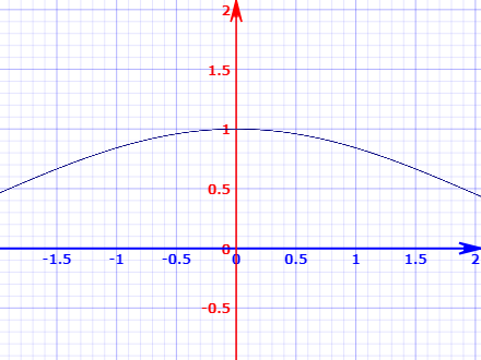
1. The function $\frac{\sin x}{x}$ appears to behave normally when $x = 0,$ as for instance in graph C-6, despite an apparent division by $0.$ Make a case for this being so.
2. When do the tangent and secant fail? What is happening with our triangle as we approach these trouble spots? What if we come from the other direction?
Adjacent, opposite, hypotenuse (C)
So far, we have been treating the triangles as rooted at the right-hand side. As we covered in the first article, often we will begin with an idealized triangle to make our points and then abstract from there.
(NOTES: images: Rotated angle -> flat base; dx-dy-r -> adjacent-opposite-hypotenuse / adj-opp-hyp)
To this end, rather than the $dx$ and $dy$ we have used thus far, these sides tend to be designated as adjacent and opposite, respectively. These have the same meanings as before, describing their relationship to the angle. This has some interesting outcomes: for instance, the adjacent side might in fact be behind us.
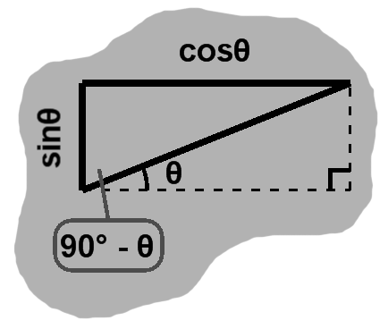
As we saw before, two congruent right triangles can be combined as a rectangle. In the first quadrant of the unit circle, this gives us the situation in figure E-3, where the angle complementary to the central angle is opposite its adjacent side and adjacent to its opposite side. Thus \begin{align} \cos(\theta - 90^\circ) = \sin\theta \\ \sin(\theta - 90^\circ) = \cos\theta \end{align}
(NOTES: this is a general thing)
(NOTES: symmetry about 45°)
Plugging in our earlier results for 30°: \begin{align} \cos 60^{\circ} & = \frac{1}{2} \\ \sin 60^{\circ} & = \frac{\sqrt{3}}{2} \end{align}
Beyond the motivation, of course, we made little use of the circles. In fact, we can simply pretend one is there, allowing us to generalize these to any situation with a right triangle.