
Today’s guest tutorial comes to you courtesy of X.
Two-dimensional geometry comes into play whenever we use Corona's display objects.
This is largely done at a high level and comes quite naturally. Assuming our code works, we rarely give statements like circle.x = 10 or
image.rotation = 30 more than a passing thought.
We might find ourselves wanting to do more, however. A broader knowledge of geometry then becomes useful, even necessary. This series aims to explore several of the fundamental ideas: how to come up with them in the first place, and then put them to work.
Some quick notes
The target audience is a reader with at least a basic grasp of arithmetic (distributive law, powers, roots). Some familiarity with algebra might also be helpful.
The material is arranged so that later sections build upon earlier ones. This will also be true from one article to the next, as the series progresses. Naturally, there is going to be a lot to absorb! Many concepts might require several rereads, as well as a bit of time—and perhaps some experimentation in Corona?—before finally sinking in, especially for someone new to it all.
For the most part, the various links are simply "further reading": alternative proofs, additional points of view, visualizations, even some history.
Similarly, some sections end with exercises, marked as YOUR TURN. These are optional as well, but working them out might offer interesting insights. While digressionary, these more closely follow the material in the text.
Mathematical expressions are rendered using the MathJax toolkit. (Punctuation characters such as periods and commas are rolled into such expressions whenever they immediately follow them; this makes the characters stand out a bit, especially when their unadorned counterparts are nearby, but eliminates some occasional formatting weirdness.)
This repository contains the various small programs, along with a few support modules, used to generate most of the figures in these articles. The mathematical ideas under discussion naturally tend to appear in the corresponding code, so it might be worth an occasional look. Be aware, however, that more advanced concepts sometimes show up as well.
Opening lines
Our first order of business is to say a little about lines.
Lines are one-dimensional objects, meaning if we want to travel along one, we only have one direction available to follow, either forward or backward. If we veer to the side, we leave the line.
Many times, we want to consider lines in connection with their surroundings, perhaps as part of another object. By doing so, we embed them in space (or "in the plane", in two dimensions). This introduces position and orientation.
(NOTES: Expand on that last bit; some of what's in "Going the distance" would be better off here)
Curves are another sort of one-dimensional object, where the local direction changes from position to position. They look like line segments up close. Lines are particular in that by going from point to point our relative positions are the same in the space itself.
Lines will go on forever. But little bits of it are important. We can bound in one direction and we get rays. Or from both sides and then we have segments.
(NOTES: The last couple paragraphs are probably the ideas we want, but written quickly and need polish.)
Discussing each side's terms
Triangles are a fitting place to begin.
As the name suggests, these are objects with three angles.
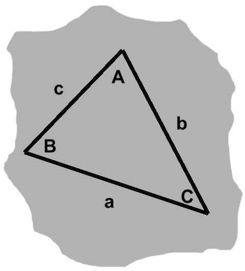
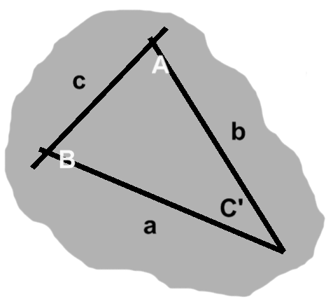
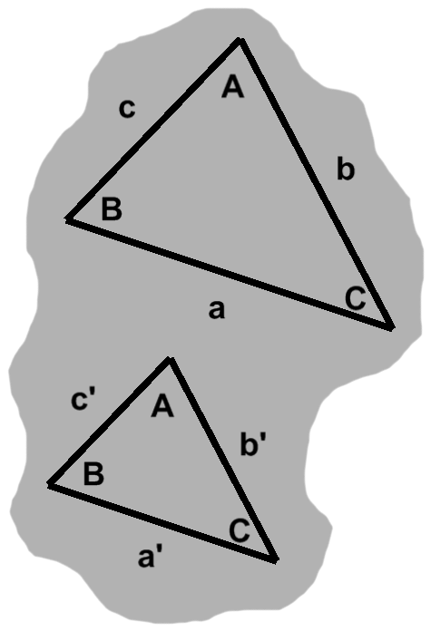
Yet this only tells us part of the story. It is equally true that a triangle is a three-sided object. A proper treatment must take both views into account. The triangle in figure A-1, for instance, has angles $A,$ $B,$ and $C,$ as well as sides $a,$ $b,$ and $c.$
There are some noteworthy relationships between angles and sides.
To begin, we might speak of a side being "across from" some angle. This relationship can be seen in figure A-1: each uppercase letter labels an angle, whereas its lowercase counterpart designates the side opposite that angle. Side $a$, for example, is opposite angle $A.$
The remaining two sides, those "next to" the angle in question, are adjacent. The angle itself is included between these sides. Continuing with our example, these would be sides $b$ and $c.$
The rather general triangle in figure A-1 might seem difficult to approach, but notice what happens if we tilt our heads to the right just a bit: side $a$ appears to be horizontal, though none of the angles have changed and all sides remain just as long.
From this perspective, certain obstacles simply go away. We suddenly have a notion of "up", for instance, suggesting avenues we might explore. This demonstrates a technique common in mathematics: we transform one thing into something simpler, perform some action on that, then reverse-transform the results.
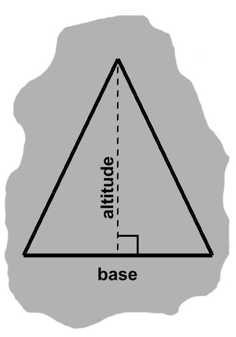
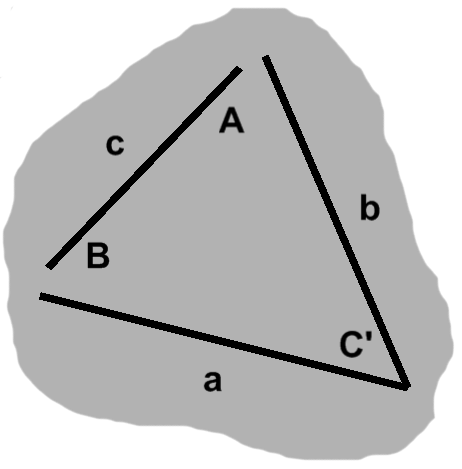
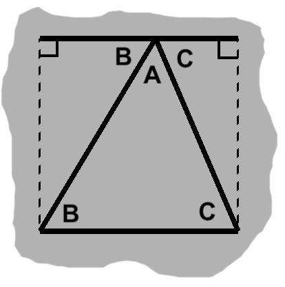
Throughout this article, for instance, we will often use "nice" triangles, such as the one in figure A-2, but these can be understood as the middle step between two rotations that happen offscreen: align one side → do our analysis → restore original orientation.
Given a horizontal side, we may draw a line segment straight up from it toward the corner which it lies opposite, the dashed vertical segments in figures A-2 and A-4 being examples. Such a segment is known as an altitude. Its length is called a height and the triangle side is a base.
Any side will do as a base, though in many problems one will stand out, for one reason or another. Each choice is paired up with a different altitude, of course.
An altitude is said to be perpendicular to its base: we have the junction of a horizontal segment with a vertical one, resulting in a right angle. Conventionally, such angles are depicted by squares. The altitude and base will often make a T when they meet, perhaps an upside-down one as in figure A-2. Naturally enough, the ⊥ symbol has come to indicate perpendicularity.
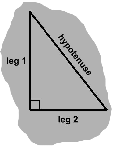
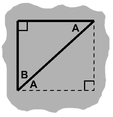
If the altitude and one of the sides overlap, we have a right triangle, as in A-3. In such a triangle, the side opposite the right angle is known as the hypotenuse. The adjacent sides are called legs.
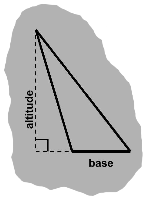
Angles wider than a right angle are said to be obtuse. (Their narrower cousins are acute.) When a base is adjacent to such an angle, both remaining sides lean either left or right, so that their corner is no longer above the base. As a result, the altitude will be outside the triangle. The base and altitude will not even meet, unless the former is extended artificially, as in A-4.
Considering different angles
In real-world situations, we will nearly always want something more precise than "wider (or narrower) than a right angle". With this in mind, angles are assigned a measure that increases in proportion to the separation between sides.
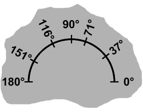
Measurements are denominated in degrees in this article, though other units are available as well. In a triangle, the range of angles begins just after 0° (sides together, thus no angle), runs through 90° (right angles), and ends a bit shy of 180° (sides fully apart, in a straight line).
Many sources label corners rather than angles, adopting a different scheme for the latter. If a triangle had corners $A,$ $B,$ and $C,$ it would be typical under these circumstances to see angles such as $ \angle ABC. $ This particular choice would refer to the angle at corner $B$ or, more specifically, included between the segment from $A$ to $B$ and the segment from $B$ to $C.$ The measure to go along with it would be written as $ \measuredangle ABC. $ For simplicity, this article will continue to label angles directly. Additionally, we will use this notation interchangeably for both angles and their measures, according to context.
By interspersing one or more lines, an angle can be divided up into two or more adjacent angles. B-2 shows such a situation. Conversely, neighboring angles may be coalesced. We can measure the full angle simply by adding up the lesser ones.
Adjacent angles share a side and corner. Thus, a given angle may be adjacent to one or two other angles, or none at all.
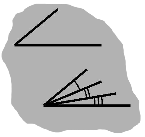
Garden-variety angles are often denoted by one or more arcs, as in figures B-2, B-3, and B-4. When two or more angles are shown with the same number of arcs, these angles are understood to have equal measurements. Varying numbers are typically a cue that the angles need not be equal (but could be). They might instead mean the angles must in fact be different, but usually this stronger condition will be spelled out.
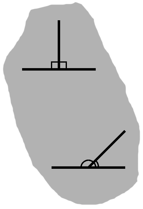
When placed side by side, two right angles will form a straight line. More generally, any two angles that do so are said to be supplementary. A pair that combine to form a right angle, on the other hand, are complementary.
Since an angle may be adjacent to an angle on each side, it might in fact be supplementary to both of them.
Furthermore, we can say the same about the supplementary angles themselves. We already know about the original angle, of course, but each one might supplement another angle, equally wide.
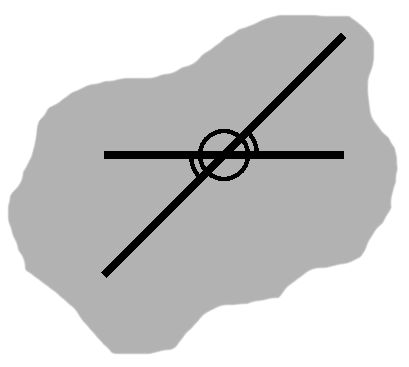
In fact, we would then have the situation of figure B-4, with the fourth and final angle being shared as well. In the end, we have a couple pairs of equal angles. These so-called vertical angles arise whenever two lines cross.
(NOTES: Loosen up a bit: describe and show a supplementary angle... then mention that we had to extend one of the sides to get the line we were completing... since an angle corresponds to two sides, we have another line, so supplementary to that as well... but the measure will be the same... we still have a fourth angle, but notice it's also flush with these lines, so has the original measure... then describe vertical, and tie it to crossing lines)
Sticking together
A little thought experiment is now in order.
Consider what would happen if, beginning with the triangle from figure A-1, we were to narrow or widen one of its angles, say $C.$ On top of this, suppose no other angle or side length was allowed to change.
Figures C-1 and C-2 depict a couple possible outcomes, following only slight variations in $C.$
A narrower angle results in the situation shown in figure C-1, where the adjacent sides, $a$ and $b$, arrive at the opposite side "early" and penetrate it—rather than meet up with its endpoints and form corners—then press on just a bit farther.
With a wider angle, on the other hand, the sides stop short of $c$, if only barely, but also veer away from it. Figure C-2 is an example of what we might see.
In order to repair one of these objects, restoring its triangularity, we would need to slide side $c$ either forward or backward, until it was in line with the endpoints of both $a$ and $b$, then either shrink or extend it for a snug fit. Barring that, neither case deserves to be called a triangle.
Small adjustments to a side length would produce similar breakage, assuming the remaining properties were held fixed.
As our short investigation shows, triangles possess a very rigid structure. Angle measures and side lengths are closely related, with only a bit of give-and-take being possible. Consequently, once a few of its angles and sides have been pinned down, so are the others. This works in our favor: knowing only some of a triangle's properties, we can deduce the rest!
When dealing with multiple triangles, this is especially important. Angles and sides will accumulate quickly; the more of them we can ignore, the better off we are.
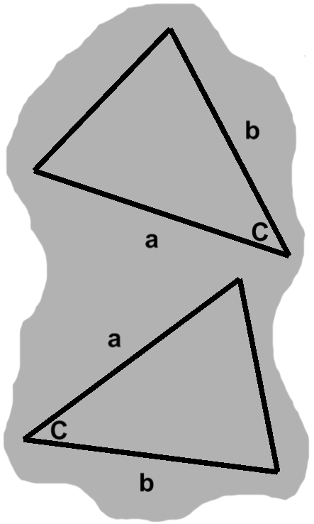
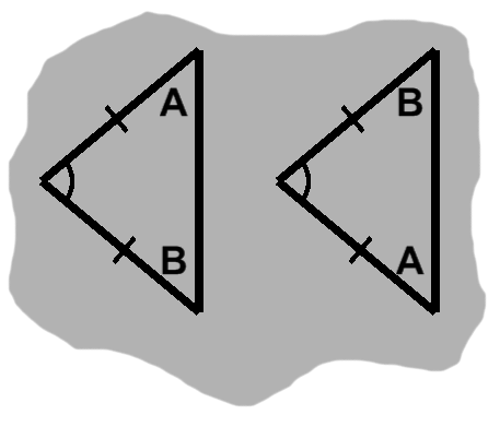
Suppose we have two triangles, $T_1$ and $T_2,$ on hand. Taking $T_1,$ we measure one of its angles plus the adjacent sides, labeling them as $C,$ $a,$ and $b$ respectively.
Say we then shifted our attention to $T_2.$ When measured, one of its angles turns out to be exactly as wide as $C.$ These things do happen, of course, so it goes unremarked.
As we measure the angle's adjacent sides, further similarities emerge: one has the same length as $a,$ the other is as long as $b.$ $T_1$ and $T_2$ have a common side-angle-side sequence. If matching parts were assigned the same labels, we have something like figure C-3.
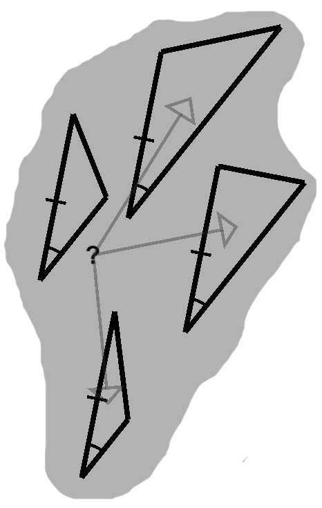
When we only knew an angle and one of its adjacent sides, $T_2$ was still quite malleable. One of its angles was still totally independent at this point. This scenario is depicted in figure C-4: the triangle may not assume any shape, since part of its structure is indeed locked down, but limitless possibilities exist nonetheless. (Slash marks serve the same purpose for sides that arcs do for angles, with matching counts indicating equal lengths.)
Introducing the second adjacent side will bring us back to our earlier predicament, where any change would upset a delicate balance. This has an extremely important converse: a common side-angle-side sequence means that two triangles are the same.
(NOTES: Is the first half of this clear? Realized it could be more intuitively demonstrated by overlap...)
EXERCISES
1. What other theorems can we use to compare triangles, based on angles and sides?
2. Do these theorems have the same guarantees as side-angle-side?
Identical twins
Properly speaking, the two triangles are congruent. This has a few (equivalent) definitions.
Suppose we have a triangle and decide to traverse its boundary. Each step of the way, we compare our current location to every other one on the same triangle, finding the distance between them. (We will soon see how to perform such calculations.)
At the same time, we examine corresponding points on a congruent triangle. In every instance, the results will be identical.
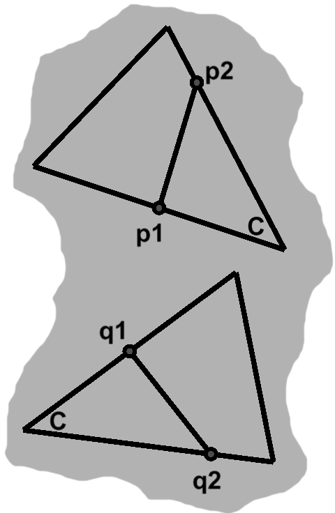
Figure D-1 is a snapshot of this process. On one triangle, we have chosen two points, $p_1$ and $p_2$, in the middle of one side and three-quarters of the way along another, respectively. On a second triangle, $q_1$ and $q_2$ are equally situated. (Corresponding sides have the same lengths, of course.) Whatever distance lies between $p_1$ and $p_2$ also separates $q_1$ from $q_2$.
When all lengths match, we have congruence. Comparing infinitely many pairs of points is impractical, to say the least, but captures what is going on numerically.
Alternatively, we may speak in terms of rigid motions. These are geometric operations that preserve an object's size and shape: changing its position, rotating it, or taking its mirror image. If we start with one triangle and are able through some combination of these motions to make it perfectly overlap another, the two triangles are congruent. In figure C-3, as an example, we can rotate one of the triangles and move it atop its companion.
The two approaches are not at odds. Overlap is the visual manifestation of all lengths being in agreement, and vice versa.
(NOTES: Either move this before the last section (with appropriate edits) or use overlap to show side-angle-side in effect)
A look in the mirror
An isosceles triangle, where two sides have the same length, shares a side-angle-side sequence with one of its own mirror images. It will therefore be congruent to this "other" triangle.
On account of common lengths, the triangle and mirror image already coincide. With some separation, they might look something like figure E-1. For the initial overlap to have been possible, angles $A$ and $B$ must be equal.
In an equilateral triangle, all sides have the same length.
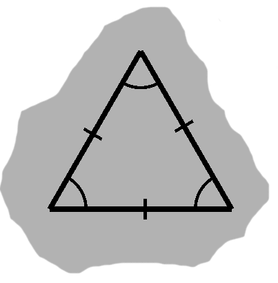
By restricting ourselves to a couple sides, we can approach this as an isosceles triangle. This will tell us that two angles are equal. Choosing another pair of sides, we can repeat the process, giving us another match. Only three angles are possible, so one of them must show up twice.
For instance, say angles $A$ and $B$ are equal in the first case, $B$ and $C$ in the second. Since they have $B$ in common, $A$ and $C$ ought to match as well. The third pair of sides will confirm this.
TENTATIVE TENTATIVE TENTATIVE TENTATIVE TENTATIVE TENTATIVE TENTATIVE TENTATIVE TENTATIVE
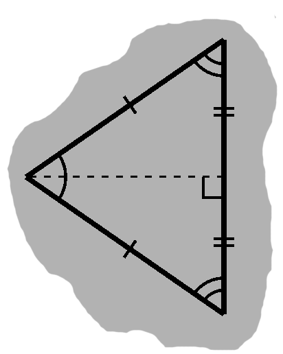
In the less specific isosceles case, we can cut the third side in half, as in E-3. In doing so, we get two triangles with a side-angle-side relationship.
Because this creates two new angles, these must be equal to one another. Since they came from what was originally a line, they must be supplementary, and thus right angles.
The new common side splits the remaining angle, as well. Since these new angles must be equal, each must measure half the original.
We call such sides perpendicular bisectors.
TENTATIVE TENTATIVE TENTATIVE TENTATIVE TENTATIVE TENTATIVE TENTATIVE TENTATIVE TENTATIVE
Drawing parallels
(NOTES: If we go the overlap route, which is likely, it seems much better to approach this using I-1 and I-2, along with the material for the same... we can still use some of what follows here... this might also let us cut some of the awkward "rectangles have parallel sides" bit in the next section)
(NOTES: The main thrust is that, because two sides already coincide as the transversal, the alternate angles situation means that the other two sides must be oriented the same way... "we call this parallel", etc.)
We have only been considering segments of lines, rather than the real deal. A segment begins in one location and ends in another, whereas lines continue in either direction indefinitely.
Lines are unbounded, but still pass through points. Selecting any two of them will give us the endpoints of a segment within the line. Conversely, the presence of a segment suggests the broader line embedding it.
Each of a triangle's three sides is a segment that can be understood as part of a line. This is rather precarious, of course: nearly any change in position will shift the side outside the line.
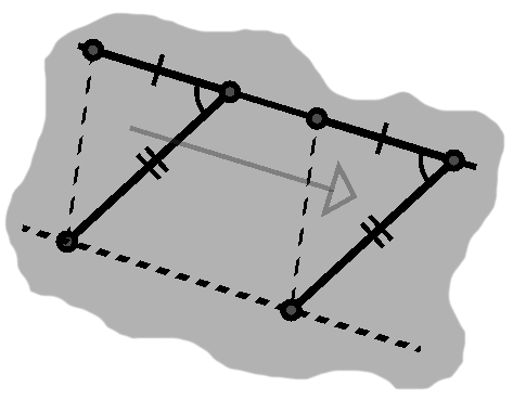
Parallel movements, however, will keep this relationship intact. These follow the direction of the line in question; the side will simply slide backward or forward along the line. If we move the entire triangle at once, we get something like figure G-1.
We can draw some useful inferences by considering the triangle before and after this movement as distinct.
Because the triangle only underwent a straight-line motion, without being flipped or rotated, its sides retain their same directions as well: the segments are parallel. For instance, this describes the two sides with double slash marks in figure G-1.
Naturally, since the sides never change direction, the angles between them are preserved as well. In fact, beyond motivating this insight, an underlying triangle is not even necessary. Whenever we have parallel segments sliced by a third one, we end up with several corresponding angles. The arcs in figure G-1 represent one of these equal pairs.
Two of the triangle's corners belong to the side embedded in the line, with the remaining one outside. When we move the triangle, however, this point traces a second line, as shown in dashes in figure G-1. Since the two share the same direction, these lines are also parallel.
Because parallel lines or segments follow the same direction, the distance between them will never change. In figure G-1, for instance, the triangles' heights—with the segments inside the line as bases, of course—will report the same distance separating the two lines. Parallel objects either never meet or completely coincide already.
EXERCISES
1. Demonstrate the midpoint theorem: if we connect the midpoint of one side with the midpoint of another, the segment between them will be half as long and parallel to the remaining side.
Triangles in space!
Given a rectangle, we might try packing it full of smaller objects.
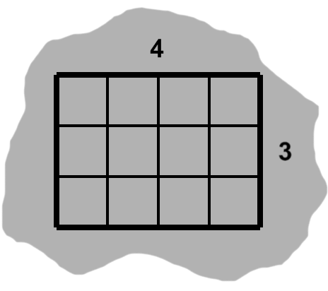
In figure H-1, we have a rectangle four units wide by three units tall. (Our unit in this case is generic, but in practice could be feet, meters, any of their derivatives, and so on.) It contains several one-by-one rectangles, or unit squares.
These squares form a grid, so we can easily count them. Each row consists of the same number of squares, so we need only multiply our column and row counts together. The rectangle in our example is able to fit twelve unit squares.
We might instead say that it has an area of twelve square units, or 12 units².
Our counting strategy holds in general. A rectangle's area is given by its width times its height, often written $ wh. $
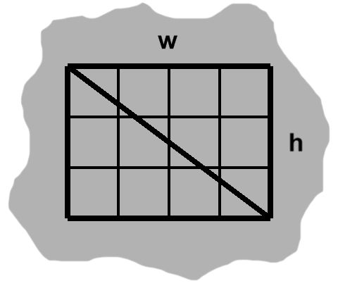
Now, if we slice a rectangle diagonally, from one corner to another, we end up with two triangles, as in figure H-2.
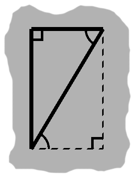
A rectangle, by definition, has four right angles. If two sides both happen to be perpendicular to a third side, they will be parallel to one another.
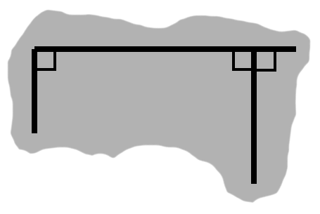
Figure H-3 demonstrates why this is so. By supplementing one of the angles, we obtain another right angle. We then have corresponding angles, which arise in the presence of parallel lines. Since this transpires in all four cases, we can deduce that the rectangle has two pairs of parallel sides: left and right, bottom and top.
Since distances remain fixed between parallel segments, it follows that a rectangle's parallel sides have equal lengths. In figure H-2, the left side is between the bottom and top sides, so it also has length $h,$ like the right side. The same holds true for the bottom and top sides with $w.$
By side-angle-side, our divided rectangle has become congruent triangles. As we know, these can be moved and rotated to overlap. Each triangle therefore occupies the same amount of space.
Area and space basically express the same idea. Each triangle has half the area of the original rectangle. An area formula for right triangles immediately follows: $ {wh \over 2}. $
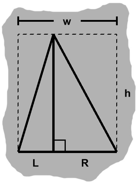
Earlier, in figure A-2, we saw that an altitude decomposes a triangle into two right triangles with shorter bases. A base $w$ units wide divides into sub-bases with widths $L$ and $R,$ as in figure H-4.
From our new formula, the areas of these child triangles are $ Lh \over 2 $ and $ {Rh \over 2}. $ Adding them together gives us a total area of $ {(L + R)h \over 2}. $ Of course, $ L + R = w, $ so the area of the original triangle is in fact $ {wh \over 2}. $
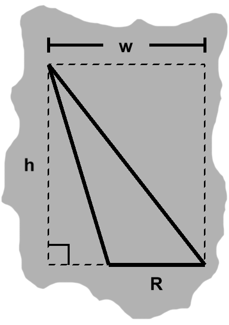
When dealing with an obtuse angle, our approach is slightly different. Assuming $w$ is still the width of the enclosing rectangle, our triangle's base will be a shorter length, $R,$ as in figure H-5.
As we saw earlier in figure A-4, the base in these cases can be extended to intercept the altitude. The augmented triangle this produces is a right triangle, with area $ {wh \over 2}. $ Furthermore, the added-on part is one as well, measuring $ { (w - R)h \over 2 } $.
The area of our original triangle will be the augmented area minus that of the extension: $ {Rh \over 2}. $ Despite a slight change of circumstances, $R$ is also the width of the base, just as $w$ was in the previous two cases.
In general, triangle area is given by $ {bh \over 2}, $ where $b$ is a base width and $h$ the corresponding height.
As an aside, with our four-by-three rectangle, we end up with two triangles of area 6 units². While this still happens to be an integer, the original packing of whole unit squares no longer corresponds to the shape: the area is now dispersed across the squares, with many of them only partially full, as a quick look at figure H-2 will tell us. This ought to provide some insight into how the notion of area generalizes.
EXERCISES
1. Use smaller squares to represent a triangular half rectangle, making sure these almost add up to the proper area. Doing this, can we ever get a perfect fit?
2. Demonstrate some examples of the distributive law geometrically.
It All Adds Up
We can also go the other way. Given a right triangle, we make a copy of it. A couple rigid motions will then bring the two together, forming a rectangle as in figure I-1.
Notice the arcs, indicating a pair of alternate angles. When one line crosses two others, we will have a Z-like configuration, with this sort of arrangement of angles around the central segment. In this example we began with congruent triangles, so the angles are equal as well.
Once again, this particular example introduces the idea, but any sort of triangle will do. In fact, the only real necessity is that we have three segments forming a Z, with two of them being parallel.
We can see why this is so in figure I-2. Even if we have a rather generic triangle, knowing its altitude will let us carve out a right triangle, at which point we can build a rectangle as before.
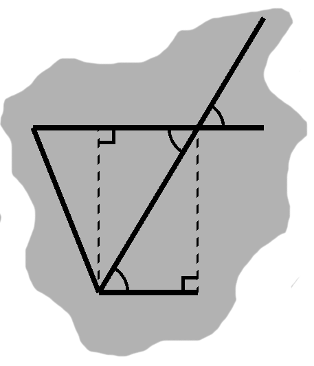
More importantly, some of our earlier concepts come together. Since we have parallel sides, we get corresponding angles as well, say $A$ and $B$. We also have a third angle that is both vertical to $A$ and alternate to $B$. We see this sort of relationship in figure I-2. We already know that corresponding and vertical angles are equal. The same must be true of alternate angles when we have parallel segments.
If we began with a fairly typical triangle, such as the one in figure H-4, we would need to add two right triangles to work our way back to a rectangle.
Doing so will tease out a pair of alternate angles from the triangle. Furthermore, these form a line with the remaining angle, as in figure I-3. Since their measures are the same as these three, the sum of the triangle's interior angles must be 180°.
This approach might seem to rule out triangles with either a right or an obtuse angle. Actually, if we turn such a triangle so that its longest side is on the bottom, we will have the previous scenario. Since the sum of angles is a feature of the whole triangle rather than a given side, we could stop here. The other possibilities are not too onerous, however, so we ought to go over them as well.
Right triangles are rather simple. Again, these are simply half rectangles, with parallel sides leading to equal alternate angles. Because it fills a corner, one of these angles will also complement the angle already found there. From figure I-4, for instance, we see that $ A + B = 90^{\circ}. $ As expected, $A,$ $B,$ and the right angle add up to 180°.
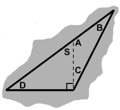
An obtuse angle, say $O,$ decomposes into a right angle and smaller adjacent angle. On their own, we already know how to attack the two triangles this gives us; a hybrid approach will get us the rest of the way.
We will have a situation like figure I-5. At the outset, we know that $ D + S = 90^{\circ} $ and $ C = O - 90^{\circ}. $ Because $S$ and $A$ form a line, the first of these can be rewritten as $ D + (180^{\circ} - A) = 90^{\circ}, $ or $ A = D + 90^{\circ}. $
Now, $ A + B + C = 180^{\circ}. $ Plugging in our recent findings, the left-hand side becomes $ (D + 90^{\circ}) + B + (O - 90^{\circ}). $ This simplifies to $ B + D + O = 180^{\circ}. $ All is well.
EXERCISES
1. What happens with four sides? Do we need to account for special cases?
2. What about the general case of $n$ sides ($n >= 3$)?
Enter Pythagoras
Squares are a special case of rectangles, where all sides have the same length.
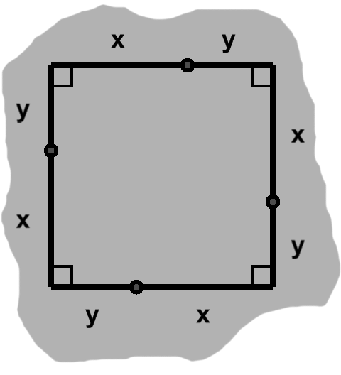
Borrowing an earlier idea, we can divide each of these sides into two lesser lengths, say $x$ and $y.$ If these alternate around the square, we have something like figure J-1.
From the rectangular formula, the total area of the square is $ (x + y) \times (x + y). $ We can expand this to get $ x^2 + 2xy + y^2. $
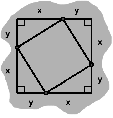
Notice the small nodes in figure J-1, wherever the sides have been split. If we visit these in sequence, drawing segments from one to the next, we etch four right triangles out of the square.
By side-angle-side, we know these triangles are congruent, each with area $ {xy \over 2}. $ The area of all four together is $ 4\left({xy \over 2} \right) = 2xy. $
We can find the area of the middle region—what would remain, if we removed the triangles—by subtracting this sum from the total area of the square. The $ 2xy $ terms cancel, leaving us with $ x^2 + y^2. $
One side of each triangle remains unknown. Owing to congruence, however, these sides all have the same length. We can give them a common label, say $z.$
The middle object's angles each lie along a side of the square; when combined with their neighbors, they form straight lines. Thus, if $A$ and $B$ are the adjacent measurements, a given angle has measure $ 180^{\circ} - A - B $.
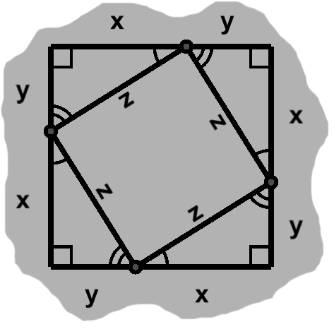
As the arcs in J-3 indicate, $A$ and $B$ will be the same in all four cases. The interior angles must therefore be equal as well, measuring $ 360^{\circ} / 4 = 90^{\circ}. $
The middle region is an equal-sided object with four right angles. This is simply a rotated square, with area $ z^2 $. A few paragraphs ago, we described this same area using another formula. We can combine the two, giving us $ x^2 + y^2 = z^2. $
This is the celebrated Pythagorean theorem.
"This base is too short..."
Now, while the central square was key to arriving at this result, the equation actually describes a relationship among triangle sides.
These happened to be right triangles during our derivation, but is this necessary? Might the formula extend to triangles in general, as with area and interior angle sums?
We run into problems right out of the gate. Without a right angle, nothing seems to distinguish any one side. Which one gets to be $z$?
Setting such practical concerns aside, consider the following candidate, depicted in figure K-1. If its base, $x,$ were somewhat wider, we would indeed have a right triangle. As is, it falls short.
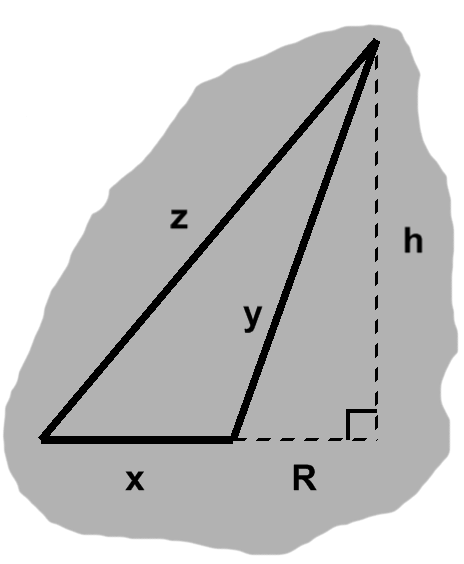
We ran across a similar predicament with areas involving obtuse angles. Once again, we can start with the "hypothetical" right triangle that a longer $x$ would give us. This has base $ x + R $ and height $h.$ Of course, it does adhere to the Pythagorean equation: $ (x + R)^2 + h^2 = z^2. $
Also familiar: the added-on part is itself a right triangle. In figure K-1, its legs correspond to the dashed segments. Thus, $ h^2 = y^2 - R^2. $
We can plug this into the previous equation. Following some expansion and cancellation, we have $ z^2 - x^2 - 2xR = y^2. $
Now, if our non-right triangle does indeed satisfy Pythagoras's equation, $ x^2 + y^2 $ will be the same as $ z^2, $ so we can substitute one for the other in the last result. A short bout of cancellation ensues and leaves us with $ -2xR = 0. $
This could mean $ R = 0 $: nothing needs to be added to $x$, so we have a right triangle after all!
Otherwise, $ x = 0. $ This is indeed suspicious.
"...this base is too long..."
The base might instead be too wide to be a right triangle, as seen for instance in figure L-1.
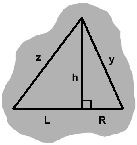
Delving once more into earlier techniques, we can draw an altitude to break this apart into two right triangles, with bases $L$ and $R$ and a common height $h.$ Applying the Pythagorean theorem to these, we find $ L^2 + h^2 = z^2 $ and $ R^2 + h^2 = y^2. $
Again, assuming the original triangle does satisfy the Pythagorean theorem, we can replace $ z^2 $ in the first equation with $ x^2 + y^2. $ Doing so, then combining the two equations on account of the common $ h^2, $ and finishing off with some cancellation, we end up with $ x^2 + R^2 = L^2. $
Since $ x = L + R, $ this finally boils down to $ 2R(L + R) = 0. $ Either $ L = -R, $ which can only happen when $ x = 0, $ or $ R = 0. $ These are exactly the situations a too-short base gave us, with the same consequences.
"...this one is just right."
The same analysis applies to $y,$ with comparable results. In short, either the solution outright demands a right triangle, or one of $x$ or $y$ must be zero. What do these latter possibilities mean?
When $x$ is zero, the equation reduces to $ y^2 = z^2, $ or $ y = \pm z. $ Similarly, with $y$ we arrive at $ x = \pm z. $ These are simply lines.
Figure M-1 gives us some hint that lines are not a drastic break from the triangular mold. So long as we have a right angle, all is well, even as the height dwindles and our triangle becomes little more than a sliver. A line segment can be understood as going just a bit further, so the height (or width of the base) is zero.
(NOTES: Perhaps a little numerical note, e.g. when $x$ is 1/1000, $x^2$ is 1/1000000, etc. so graceful transition)
So, given $x$, $y$, and $z$ satisfying the Pythagorean theorem, we know these do entail a right triangle, or might as well.
EXERCISES
1. What if $x$ and $y$ both go to zero?
2. How long can the hypotenuse be, compared to its legs?
Going the distance
All well and good, but what do we gain from the theorem?
Basically, knowing how long two sides of a triangle are, we can find the third as well. The hypotenuse is the most obvious choice: $ z = \sqrt{x^2 + y^2}. $ If we already know $z,$ we can find one of the leg lengths instead, say $ x = \sqrt{z^2 - y^2}. $ (Negative roots are irrelevant.)
Consider the two points depicted in figure N-1.
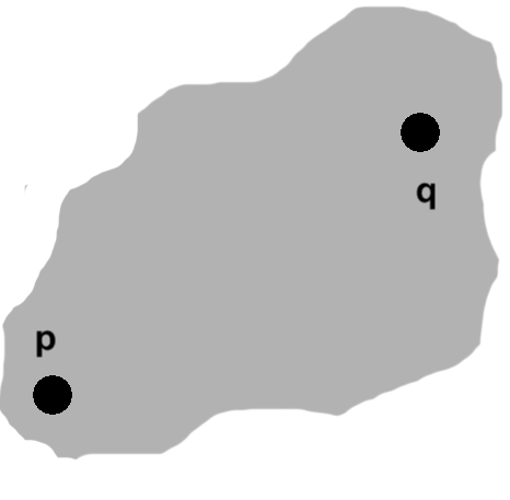
Both can be described by a coordinate pair: $ \vcomps{p_x}{p_y} $ for $ \mathbf{p} $ and $ \vcomps{q_x}{q_y} $ for $ \mathbf{q}. $ Given some point of reference, the $x$- and $y$-coordinates tell us how far to the right of and above it these points are found. For example, $ (1, -3) $ would be one unit to the right and three units below.
Rather than travel in a straight line from one point to the other, we can start from $ \mathbf{p} $ and head right, eventually putting us directly beneath $ \mathbf{q}. $ From there, going straight up will get us the rest of the way.
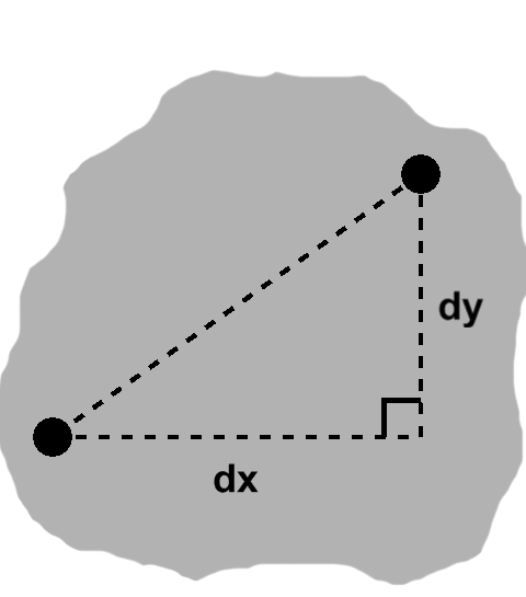
To perform these intermediate steps, we need to know "Relative to $ \mathbf{p}, $ how much farther to the right and above is $ \mathbf{q} $?". The coordinate differences express exactly this: $ dx = q_x - p_x $ and $ dy = q_y - p_y. $
Taken together, these shorter paths are the legs of a right triangle, as seen for instance in figure N-2. Its hypotenuse is the segment from $ \mathbf{p} $ to $ \mathbf{q}. $ Finding the length of this side will give us the straight-line distance between the two points: $ \sqrt{dx^2 + dy^2}. $
TENTATIVE TENTATIVE TENTATIVE TENTATIVE TENTATIVE TENTATIVE TENTATIVE TENTATIVE TENTATIVE
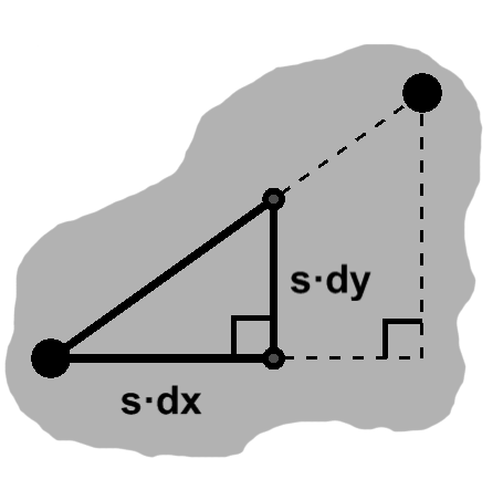
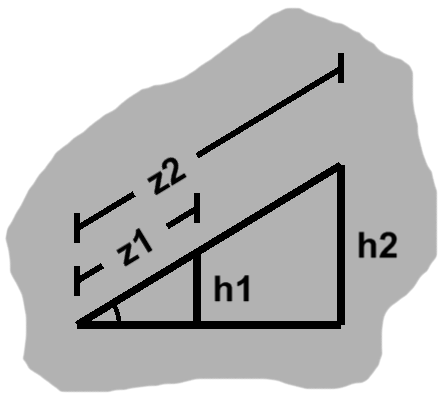
Returning to an earlier point, we mentioned that a similar triangle entailed uniformly scaling the sides of a triangle.
(NOTES: similar triangles moved after this, so revise)
In the case of a right triangle, this is pretty easy. We have two sides of length $dx$ and $dy,$ which we can scale by $s.$ Then the length of the third side would be $ \sqrt{(sdx)^2 + (sdy)^2} = \sqrt{s^2(dx^2 + dy^2)}. $ This simplifies to $ s\sqrt{dx^2 + dy^2}, $ which is exactly what we would expect.
(NOTES: A little too "lucky"; turn the steps around instead)
This applies to triangles in general, but a useful consequence follows when we apply it to distance. Basically, to find the position $s$ of the way along the path between two points, simply scale the two offsets $dx$ and $dy$ by $s,$ then add the results to the original point. This is called linear interpolation.
Importantly, the construction $ a + s(b - a) $ can be rephrased as $ (1 - s)a + sb, $ which is sometimes more convenient.
(NOTES: General triangle could use the implicit lerp triangles)
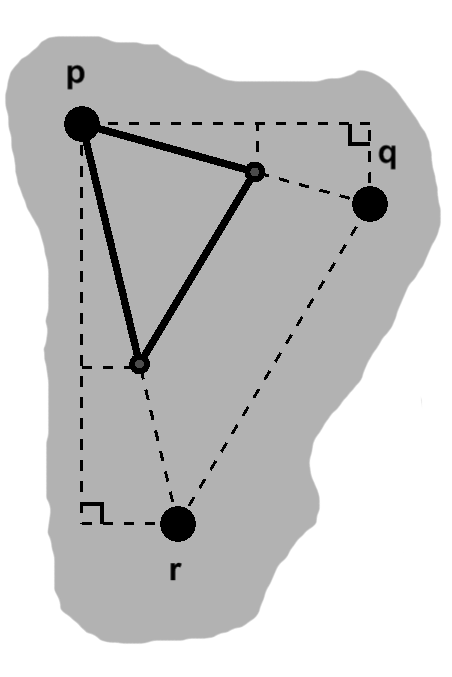
In the more general case, we can choose two of the sides with a common first point and scale them. This is simply the right triangle situation. The third side will depend on the second point, with offsets $ dx_2 = r_x - q_x, dy_2 = r_y - q_y,$ and length $ \sqrt{dx_2^2 + dy_2^2}. $
The second points on this scaled triangle will be at $ \vcomps{(1 - s)p_x + sq_x}{(1 - s)p_y + sq_y} $ and $ \vcomps{(1 - s)p_x + sr_x}{(1 - s)p_y + sr_y}. $ If we find the offsets between these points, the $ 1 - s $ terms cancel and we have $ dx_3 = s(r_x - q_x) $ and $ dy_3 = s(r_y - q_y). $ These are the scalar multiples of $dx_2$ and $dy_2,$ as expected.
(NOTES: More complex than necessary... just split a generic triangle into two right triangles, aligned along the altitude for visual clarity... then to get the two "hypotenuse" sides we scale the legs... since this altitude is a leg of both, we use the same scaling factor, and since s(x + y) = sx + sy, the bases are the same too, so all checks out)
Strikingly similar
Had congruence been the only way to relate two triangles, giving it a special name would be redundant. There is, in fact, another useful concept of "same".
Say we came across the two triangles in figure F-1.
One triangle is visibly smaller than the other, so overlap is clearly not going to happen. That said, both triangles have the same set of angles. In spite of the size difference, the shapes match. (Once we know how to find lengths, we could show that one triangle is simply a scaled version of the other.)
The two triangles are said to be similar.
Similar triangles, like congruent ones, may have different positions and orientations. Two triangles might even share a corner—and thus an angle—so that the smaller triangle is "part of" the larger one, as seen in figure F-2. Naturally, the shared angle would be the same as itself!
(NOTES: For F-3, use variant of F-1; two sides on one of them, one plus a "?" on the other; maybe rotate it for increased generality)
(NOTES: In fact, could strengthen this by swapping with next section; motivate by overlap case and corresponding angles)
(NOTES: Still needs a little finesse to tie in the uniform scaling; perhaps the better-elaborated rigidity section earlier?)
TENTATIVE TENTATIVE TENTATIVE TENTATIVE TENTATIVE TENTATIVE TENTATIVE TENTATIVE TENTATIVE
EXERCISES
1. Make an argument for similarity from the midpoint theorem, mentioned in an earlier exercise.
2. If we know two triangles are similar, how can we take of advantage of this by scaling one or both of them? What about rotating? Scaling and rotating? As far as rotation goes, consider that the triangles might be doing so around different centers.
Summary
There is much more to be said about triangles. Even so, what we have already is nothing to scoff at. Naturally, the most obvious results, such as which angles are the same and how to measure areas, are important. The assortment of techniques used along the way are also well worth remembering, as they tend to come up again and again.
Future articles will build upon this foundation. Next up: circles!