
Today’s guest tutorial comes to you courtesy of X.
In the previous entries of this series, we looked at triangles and circles. This time around, we explore the idea of vectors.
The present article enlarges upon many points made in parts 1 and 2, so interested readers are advised to begin with those.
Vectors (A)
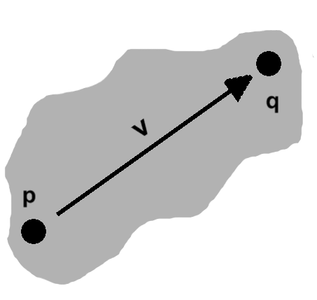
Our study of triangles concluded with a short look at distances. In doing so, we used two representations of points: as objects in their own right, named $ \mathbf{p} $ and $ \mathbf{q} $ in the text, or as bundles of components, $ \vcomps{p_x}{p_y} $ and $ \vcomps{q_x}{q_y} $. These are largely interchangeable, though different situations tend to better suit one or the other. Generally, we favor the whole point approach unless something about the individual components calls for our attention.
While deriving the distance between $ \mathbf{p} $ and $ \mathbf{q} $, the values $dx$ and $dy$ showed up, these being the differences of the points' $x$ and $y$ components, respectively. These can be bundled as well, as $ \vcomps{dx}{dy} $, and given a collective name, say $ \mathbf{v} $.
Now, we subtracted the components of $ \mathbf{p} $ from those of $ \mathbf{q} $. Had we done it the other way around, we would have a slightly different pair: $ \vcomps{-dx}{-dy} $. That is to say, $ \mathbf{v} $ has a built-in sense of direction. This is rather unintuitive with respect to points; conceptually, $ \mathbf{v} $ seems to be another sort of object, namely a vector.
Often these will be written with an arrow up top, as $ \vec{v} $ or $ \vec{\mathbf{v}} $. This article will stick to mere boldface.
Given which components we subtracted from which others, it seems that we could get away with saying $ \mathbf{v} = \mathbf{q} - \mathbf{p}. $ Assuming known rules of arithmetic hold, we could even rearrange this as $ \mathbf{p} + \mathbf{v} = \mathbf{q} $ or $ \mathbf{p} = \mathbf{q} - \mathbf{v}. $
Following the lead of our motivating example, in adding a point and vector, we add the $x$ and $y$ components of each separately, assigning the respective sums to those same components in a new point: $ \vcomps{p_x}{p_y} + \vcomps{v_x}{v_y} = \vcomps{p_x + v_x}{p_y + v_y}. $
Subtraction, which is essentially finding $dx$ and $dy$, proceeds identically, albeit as point minus point: $ \vcomps{q_x}{q_y} - \vcomps{p_x}{p_y} = \vcomps{q_x - p_x}{q_y - p_y}. $
If we slog our way through the vector equations component-wise, everything does indeed check out.
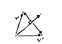
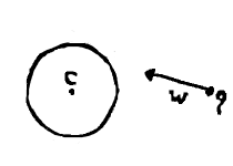
Vectors are often interpreted as paths between two points, as pictured, or displacements from some position. By definition, however, they need only be some object having both a direction and magnitude. (Consider linear velocities and forces, for instance, where physical properties come along for the ride.)


Worth noting is that the definition says nothing about position. Our considerations thus far have looked on them as auxiliary to points, but we can equally well combine vectors with one another. On the left, adding vectors $ \mathbf{v} $ and $ \mathbf{w} $ gives us resultant $ \mathbf{v + w} $. On the right, $ \mathbf{v} + (\mathbf{w - v}) $ sums to $ \mathbf{w} $.
Only certain combinations have been considered in our arithmetic; we did not add points to points, for instance. In fact, a sort of "arithmetic of types" underlies these operations. Imagine our objects carrying around a "type": zero for vectors, one for points. Furthermore, every arithmetic operation, in addition to mixing the objects' components, also determines the type of the result. Some examples:
\begin{align} point + vector &= 1 + 0 = 1 \rightarrow point \\ point - point &= 1 - 1 = 0 \rightarrow vector \\ vector + vector &= 0 + 0 = 0 \rightarrow vector \end{align}
Many combinations give us unknown types, though, such as
\begin{align} point + point &= 1 + 1 = 2 \rightarrow ??? \end{align}
We can rule these possibilities out.
Distinctions aside, points will occasionally be treated as vectors, in what follows. These can be interpreted as the point, say $ \mathbf{p} $, minus the origin $ \vcomps{0}{0} $.
Magnitude (B)
In the vectors we have been considering, magnitude means the Euclidean distance from one end (the tail) to the other (the head). This ought to be obvious when, as in the previous section, the vector is shown between two points, being the distance between them. The only novelty here is in considering length apart from a fixed position. We denote this magnitude—from here on out, we will say vector length—by double bars around the name, say as $ \vlen{v} $.
(NOTES: Some of this is redundant in light of the lerp material at the end of triangles)
Knowing how long a vector is, a natural next step is to shorten or extend it. This is achieved easily enough: a vector $s$ times as long has length $ {\mid s \mid}\sqrt{v_x^2 + v_y^2} $. This may be rolled back a bit, to $ \sqrt{s^2}\sqrt{v_x^2 + v_y^2} $ and then $ \sqrt{\left(s v_x \right)^2 + \left(s v_y \right)^2} $. In words, the scale factor simply distributes across components, so $ s\mathbf{v} = \vcomps{sv_x}{sv_y}. $ This vector has the same direction as $ \mathbf{v} $, but is shorter when $ s \lt 1 $ and longer when $ s \gt 1 $.
Note the absolute value of $s$ above. It is perfectly reasonable for $s$ to be negative, so that the vector points away from $ \mathbf{v} $: it then has the opposite sense. The length itself, however, is always positive.
Now, say we have a vector $ \vlen{v} $ units long. What happens if we scale it to be $ 1 \over \vlen{v} $ times as long?
The scaled vector has a length of one, of course! We call these unit vectors, and this particular scaling normalization. It is often much more practical to work with vectors in this form. Such vectors are often written with hats, say as $ \hat{\mathbf{u}} $.
As an immediate application, consider the case where we want a vector to have a specific length, $L$. If the original vector were one unit long, we would just scale it by $L$. In the general case, we need only normalize the vector beforehand and will never know the difference. In fact, we can even pack the two scale factors together as $ L \over \vlen{v} $ and perform everything in one step.
It must be noted that when a vector has a length of zero, or close to it, normalization is nonsensical. In a program this will manifest as a vector with huge or infinite components (and this will propagate through any operations using them). Where such vectors might arise, we should include checks that they have at least some minimum length (or squared length), and only in that event proceed with the code in question.
(IMAGES: 4, 5)
The dot product (C)
Earlier, we alluded to the vector $ \mathbf{w - v} $. From the picture, we see that it completes a triangle begun by vectors $ \mathbf{v} $ and $ \mathbf{w} $. Its length is $ \sqrt{\left(w_x - v_x \right)^2 + \left(w_y - v_y \right)^2} $; expanding the terms inside this root gives us $ w_x^2 - 2v_x w_x + v_x^2 + w_y^2 - 2v_y w_y + v_y^2 $.
Parts of this ought to look familiar. $ v_x^2 + v_y^2 $ is the squared length of $ \mathbf{v} $. Likewise for $ \mathbf{w} $. A bit of rewriting gives us $ \vlen{v}^2 + \vlen{w}^2 - 2(\dotp{v}{w}) $. This has a sum of two squares, almost making it compatible with the $ x^2 + y^2 = z^2 $ format we know from the Pythagorean theorem. When $ \dotp{v}{w} = 0, $ in fact, it will be in exactly that form.
This construction, $ \dotp{v}{w} $, is the so-called dot product, often written as $ \dotvw{v}{w} $.
Before we proceed, consider a vector that is the sum of two vectors, such as $ \mathbf{v} = \mathbf{a} + \mathbf{b} $. In component form, $ \softerdotvw{\vcomps{a_x + b_x}{a_y + b_y}}{w} = \dotp{a}{w} + \dotp{b}{w}. $ The dot product distributes! The same will be found for $ \mathbf{v} = \mathbf{a} - \mathbf{b}. $
We will need a couple other useful properties as we go on, which can be similarly verified: $ \dotvw{v}{w} = \dotvw{w}{v} $ and $ \dotvw{v}{v} = \vlen{v}^2. $
To those familiar with slopes, this ought to seem familiar. When two lines are perpendicular, the slope of one is the negative reciprocal of the other; this is the same phenomenon. (The vector form is robust against horizontal and vertical lines, though, where slopes run aground.)
(NOTES: join)
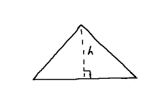
Consider a non-right triangle. As we saw in part 1, any altitude will separate this into two right triangles. The altitude gives these two triangles a common height, $h$.
Now, imagine some vectors incorporated into the mix: one of them, say $ \mathbf{v} $, sits atop the hypotenuse of one of the right triangles, while its companion, $ \mathbf{w} $, overlies the original base. These are just sides, of course, so there is an angle between them.
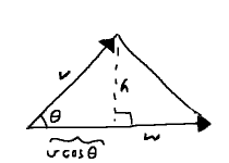
In part 2, we saw how, at any given angle $\theta$ in a circle of radius $r$, we would have a right triangle where $ dx = r\cos\theta $ and $ dy = r\sin\theta. $ We have two of the ingredients: right triangle and angle. Interpreting the hypotenuse, $ \vlen{v} $, as a radius, completes the picture. Reading things back into our triangle, then, it has base $ \vlen{v}\cos\theta $ and height $ \vlen{v}\sin\theta $.
This base uses up part of the full length, $ \vlen{w} $. The other right triangle gets the leftovers: $ \vlen{w} - \vlen{v}\cos\theta $. The Pythagorean theorem glues the remaining bits together: $ (\vlen{w} - \vlen{v}\cos\theta)^2 + h^2 = \vlen{w - v}^2. $
The right-hand side is what was used in the dot product, whereas we can FOIL much on the left. A couple terms cancel as well, and we get $ h^2 - 2\lenvw{v}{w}\cos\theta + \vlen{v}^2\cos^2\theta = \vlen{v}^2 - 2(\dotvw{v}{w}). $ After subtituting $ \vlen{v}\sin\theta $ for the shared height $h$, the left-hand side contains $ \vlen{v}^2(\cos^2\theta + \sin^2\theta) $. As we saw in part 2, the parenthesized part is exactly one. This sets off a short spree of cancellation, culminating in $ \lenvw{v}{w}\cos\theta = \dotvw{v}{w}. $
Typically one last rearrangement follows: $ \cos\theta = {\dotvw{v}{w} \over \lenvw{v}{w}}. $ The dot product associates two vectors with the angle between them. This is extremely important.
The perp operator (D)
When the Pythagorean form is satisfied, we know that we have a right angle. So we immediately find a useful application of the dot product: a result of zero means the two vectors are perpendicular. (A synonym, orthogonal, is quite common as well.)
Now, $ v_x v_y - v_x v_y = 0. $ This would seem almost too obvious to mention, but notice how closely it resembles a dot product.
In fact, it is one, albeit without the nice pairing of $x$ and $y$ labels: $ \vcomps{v_x}{v_y}\cdot\vcomps{-v_y}{v_x} $ and $ \vcomps{v_x}{v_y}\cdot\vcomps{v_y}{-v_x} $ both resolve to the left-hand side.
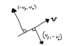
Notice what this is saying. Given a vector $ \mathbf{v} = \vcomps{v_x}{v_y}, $ we have all we need to obtain another vector, $ \mathbf{v^{\perp}} $, perpendicular to it: just swap the components and flip one of their signs. Some sources call this the perp operator.
(NOTES: Something about fixed relative orientation; CW/CCW as per rejection)
(NOTES: Successive application of operator... could bring up in last few sections about intersection)
Projection (E)
The dot product makes no assumptions about its vectors. They may point anywhere, yet it holds.
Consider again vectors $ \mathbf{v} $ and $ \mathbf{w} $ from the last section, and the right triangle arising from them with base $ \vlen{v}\cos\theta $.
As we just discovered, we can extract the cosine (without ever needing to know the angle!) from the dot product. Thus, the base length may also be written as $ {\vlen{v}(\dotvw{v}{w}) \over \lenvw{v}{w}} = {\dotvw{v}{w} \over \vlen{w}}. $
This is the component of $ \mathbf{v} $ in the $ \mathbf{w} $ direction, or $ \mathbf{comp_w v} $, which says how much of $ \mathbf{v} $ can be described by $ \mathbf{w} $. We will run into it again shortly and develop this idea a bit further.
As we have seen a couple times now, it is often useful to use vectors aligned with one of a triangle's side. As far as the base goes, it will have the same direction as $ \mathbf{w} $. Generally, $ \mathbf{w} $ will not be a unit vector, so this calls for the process alluded to earlier: normalize $ \mathbf{w} $, then scale the result to the base length. Taken together, we have a scale factor of $ \dotvw{v}{w} \over \vlen{w}^2 $. It is also not unusual to see this written as $ \dotvw{v}{w} \over \dotvw{w}{w} $, although the two forms are interchangeable.
The vector $ \left(\dotvw{v}{w} \over \dotvw{w}{w} \right)\mathbf{w} $ is known as the projection of $ \mathbf{v} $ onto $ \mathbf{w} $, or $ \mathbf{proj_w v} $. It gives us the vector "below" $ \mathbf{v} $ on $ \mathbf{w} $, its shadow as it were. (TODO: image)
(IMAGE: 9)
The projection coincides with the base of the triangle. Were we to follow the neighboring side upwards, we would get back to $ \mathbf{v} $. We can easily find this vector, the so-called rejection of $ \mathbf{v} $ from $ \mathbf{w}, $ by subtraction, following the examples in earlier images: $ \mathbf{v} - \mathbf{proj_w v} $.
As an aside, while we can go from $ \mathbf{w} $ to $ \mathbf{v} $ via addition, if we instead subtract the rejection from $ \mathbf{w}, $ we end up reflecting $ \mathbf{v} $ across $ \mathbf{w} $: $ \mathbf{v'} = \mathbf{proj_w v} - (\mathbf{v} - \mathbf{proj_w v}), $ or more simply $ \mathbf{v'} = 2 \mathbf{proj_w v} - \mathbf{v}. $ (TODO: image)
This is a vector perpendicular to $ \mathbf{w} $, along the lines of the perp operator. In that case, however, the right angle is either clockwise or counter- lockwise with respect to $ \mathbf{w} $, depending upon which definition of perp was chosen. The rejection, on the other hand, always points toward $ \mathbf{v} $. We now have the whole triangle expressed in terms of vectors.
(NOTES: Move the clockwise/CCW stuff up into perp)
Similarity (F)
Recall some of the properties of cosine, as we saw in part 2.
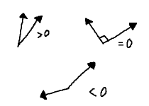
When the angle is small, the cosine's value is close to one. Near right angles, the value approaches zero. With more or less semicircular arcs, the value comes to about negative one. Any other angle falls somewhere in between. On account of cosine's symmetry, this holds both for negative and positive angles.
For this reason, the cosine, and by extension the dot product, offer a sort of similarity measurement between vectors. When two unit vectors are nearly aligned, their dot product is close to one. They are approximately the same. On the other hand, vectors perpendicular to one another have, in some sense, nothing in common, answering to values near zero. Negative products, finally, correspond to vectors facing in more or less opposite directions, completely so for negative one—they are related, but in a "everything my neighbor does, do the opposite" fashion.
(NOTES: Component for non-unit vectors)
This is a key component of many lighting models, for instance. Every point on an object's surface has a unit vector, the normal, perpendicular to it. In addition, each point looks toward the light source (rather, the light arrives from it, but we use the reverse of this direction). At each point we see compare the normal and "look at" direction. The more directly light hits, the more alike these are, and consequently the brighter that spot. The object gets steadily darker as the similarity tapers toward zero, negative values being rejected outright. For examples in Corona, see the directional or point light-based normal map effects. (TODO: image)
It was hinted earlier that we are only dealing with a fairly specific sort of vector, namely those belonging to plane geometry. Similarity hints at other uses we might explore, as well as how cosine might be applied outside a strictly geometric context. Identifying properties like similarity and teasing out their useful implications is also key to generalizing geometric operations, the dot product among them.
(IMAGE: 12)
Determined to take a side (G)
A shortcoming of the dot product, by way of the underlying symmetry, is that we cannot say which side one vector lies on relative to the other. The vector $ \mathbf{v} $ and its reflection seen in the last section, for example, are equally similar to $ \mathbf{w} $, despite their obvious differences.
Similarity does give us a way to approach this, however. Asking "Which side is this vector on?" is much like wondering "How is it similar to a perpendicular vector?". We know of two candidates here: the perp operator and the rejection. The rejection is worthless in this situation, since it always points toward the vector—yes, the rejection gets rejected—but the perp operator gives us exactly what we need, owing to its reliable orientation.
The question thus boils down to "How similar is this vector to the result of the perp operator?". $ \dotvw{v}{w^{\perp}} $ yields one sign on one side of $ \mathbf{w} $, the reverse on the other, or zero should the vectors align. (Which sign is which, of course, is subject to our choice of perp operator.)
(NOTES: join)
Both the projection and the result of the perp operator are perpendicular to $ \mathbf{w} $. Either they have the same or opposite directions; they are perfectly similar or dissimilar, pending normalization. If we call the angle between them $\phi$, we can say $ \cos\phi = \pm 1. $
Consider their dot product: $ \dotvwparen{w^{\perp}}{v - proj_w v} $.
As pointed out earlier, dot products distribute over subtraction, so this may be rewritten as $ \dotvw{w^{\perp}}{v} - \dotvw{w^{\perp}}{proj_w v} $. Also mentioned was that $ \mathbf{proj_w v} $ has the same direction as $w$—basically, $v$ gets flattened onto it. As such, it will $ \mathbf{w^{\perp}} $ is perpendicular to it as well. This makes their dot product zero, of course, leaving us with $ \dotvw{w^{\perp}}{v} $. Interestingly, this is precisely our "above or below?" similarity condition.
So long as we stay consistent, the choice of perp operator is fairly arbitrary. Selecting one and working out the components, then: $ \softerdotvw{\vcomps{w_y}{-w_x}}{v} $, or $ v_x w_y - v_y w_x $.
This is the determinant. As noted, this is equal to the earlier similarity, whose sign tells us what side $ \mathbf{v} $ lies on with respect to $ \mathbf{w} $.
(IMAGE: 13)
(NOTES: join)
Now, $ \mathbf{w^{\perp}} $ simply swaps the components $ \mathbf{w} $ and changes one of their signs. All of this comes out in the wash when we take its length, meaning $ \vlen{w^{\perp}} = \vlen{w}. $
From the dot product-cosine connection, we saw that $ \lenvw{v}{w}\cos\theta = \dotvw{v}{w}. $ At this point, we have accounted for everything except one of the vector lengths. So what is $ \vlen{v - proj_w v} $?
Of course, we could just grind it out, although the results will not be terribly enlightening. Instead, review the image of the rejection above, then recall the aforementioned dot product-cosine derivation, in particular where the right triangle's height was found. The rejection is exactly the side in question, so it follows that it has length $ \vlen{v}{\mid\sin\theta\mid} $. Note the absolute value; sine will go negative if the angle does, whereas lengths are positive. (In a right triangle, the non-right angles cannot get very wide, so negative cosines are a non-issue.) (TODO: image?)
Assembling all of this: $ \pm\vlen{w}\vlen{v}{\mid\sin\theta\mid} = v_x w_y - v_y w_x. $
The ± out front renders this somewhat unwieldy. Thankfully, $ \pm{\mid\sin\theta\mid} $ simplifies to $ \sin\theta $; sine has the aforementioned ability to go negative, so all is well. In the end, we have a sort of companion to the dot product-cosine equation: $ v_x w_y - v_y w_x = \lenvw{v}{w}\sin\theta. $
(IMAGE: 14)
(NOTES: join)
Our analysis thus far has considered vectors overlain on the sides of a right triangle. But several times, we came up with this triangle by decomposing a more general triangle. We can work backward from this insight, interpreting the side with sine-based length as an altitude. The other leg was already a projection in in the last few sections; with that in mind we can just call the full base $ \mathbf{w} $.
As we saw in part 1, the area of a triangle is $ wh \over 2 $. In our vector-sided context, this becomes $ {\lenvw{w}{v}\sin\theta} \over 2 $.
This is almost exactly the determinant, of course. It tells us that the determinant is equal to twice the area of the triangle described by two vectors, say $ \mathbf{v} $ and $ \mathbf{w} $. A doubled area is rather awkward, but we can introduce a second triangle to account for it. If we then rotate this clone and affix it to the original, we end up with a parallelogram, an object with two pairs of parallel sides. (TODO: image)
Quite often, the determinant is phrased in these terms instead, as the area of such a parallelogram. For instance, in the case of matrices and linear transformations, this more naturally mirrors the underlying coordinate systems.
(IMAGES: 15, 16)
Point in triangle (H)
Something strange is going on. We want to all that trouble getting the determinant's sign squared away, then it shows up in a formula for area! What does a negative area even mean?
First things first, the absolute value of this area carries the usual, intuitive meaning of the space taken up by the triangle or parallelogram. No surprises here.
The determinant was the same as the "which side?" similarity and also lends its sign to this area. The upshot of this is that the area's sign likewise conveys this side information. This is a bit of an odd pairing: area and side. Where might we put it some use?
In formulating the determinant above, we used the choice of perp operator that says one vector, say $ \mathbf{v} $, is on the positive side of the other, say $ \mathbf{w} $, when oriented counterclockwise to it. This is the so-called right-hand rule: starting with our fingers aligned to one vector, we rotate them to align with the other, all the while keeping our thumb pointing up; a positive angle proceeds from $ \mathbf{w} $ to $ \mathbf{v} $ is described by the right hand, otherwise the left. (TODO: images)
(NOTES: Breaks up the flow? Put the rule part in the perp operator section, maybe.)
(NOTES: Arggh, at any rate, this is proving hard to organize...)
Now, imagine a triangle, with vectors along its sides, oriented so they traverse a loop around its sides. Furthermore, this triangle contains a point. From each side, we can trace another vector toward this point, starting from the tails of these side vectors.
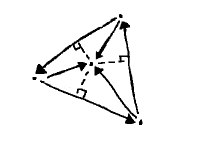
Each of the tail-to-point vectors are obviously above their respective sides, according to our right-handed convention. This will not be so, however, for a point outside the triangle, as seen on the right: on some sides the determinant is positive, on others negative, or zero when the point is on the side. Thus, we can establish containment for a point by checking that all three are positive. (TODO: image)
Together, a side and its tail-to-point vector describe a triangle, nested inside the larger one. For that matter, the implicit third side coincides with the tail-to-point vector of the next side in the sequence, so these constitute the full triangle. It seems only natural that these individual areas should sum to the total amount. (TODO: image)
These same circumstances prevail when the point lies outside the larger triangle, however, so we find ourselves in a bit of a quandary. As the picture shows, the pieces make up a larger object: the sum is not greater than its parts! Must we restrict ourselves to the inside case?
These triangles, being vector-sided, are amenable to the new area formula. These areas can be positive or negative, of course. This accounts for the extra space: whenever one of the triangles is "too positive"—the point is "above" its base, but so much it spills out of the larger triangle—another one makes up for it by having negative area—here, the point is "below" the base. In the end, the signed areas do indeed sum to the (positive) area of the full triangle.
(IMAGES: 18, 19)
Throwing one's weight around (I)
We may divide the smaller areas by the larger one, giving us three values, say $b_1$, $b_2$, and $b_3$, that sum to one. Some interesting facts follow on this. As before, points "above" a side have positive sign and those "below" negative. Then there are those on the side itself: here the "sign", or rather the value $b_i$, is zero. Consequently, the corresponding triangle vanishes: it has no area.
The point might also fall on two sides: at one of the corners. Another triangle vanishes. Two areas went to zero, so we have something like $ b_1 = b_2 = 0 $ and $ b_3 = 1. $ At each of the corners, one of the values will be one, the others zero.
When only one of the values was zero, with the point somewhere along one of the sides, the two that remain must still sum to one. Because of the situation prevailing at the corners, it seems reasonable that the nearer this point comes to a corner, the closer one $b_i$ will be to one, the other to zero. In other words, these seem to be a sort of weight, describing relative proximity to each corner. In the interior, all $b_i$ are between zero and one, but the idea still holds. Outside the triangle it does as well, though some $b_i$ will not be positive, and "on the side" might mean rather being on its infinite line.
These are barycentric ("center of weight") coordinates. (TODO: image)
These coordinates, where values of one select a corner and reject the others, suggest that a point can be described by a formula such as $ b_1\mathbf{p} + b_2\mathbf{q} + b_3\mathbf{r} $. In doing so, though, we find ourselves adding points, seemingly at odds with our earlier "arithmetic of types" guidelines.
We can see that no such violation takes place by rephrasing a couple of the points using vectors: $ \mathbf{q} = \mathbf{p} + \mathbf{v} $ and $ \mathbf{r} = \mathbf{p} + \mathbf{w}. $ The formula then becomes $ b_1\mathbf{p} + b_2(\mathbf{p} + \mathbf{v}) + b_3(\mathbf{p} + \mathbf{w}) $. After distributing the scale factors, this restructures as $ (b_1 + b_2 + b_3)\mathbf{p} + b_2\mathbf{v} + b_3\mathbf{w} $.
The parenthesized values sum to one, so the "scaling" leaves the point as is. The remaining terms are scaled vectors, which add to points just fine. Barycentric combinations are point-vector sums in disguise. (For that matter, if scaling a point also scales its "type"—making it equal to the scale factor—then although this intermediate result is some alien object, so long as the "types" all sum to one we will again have a point after adding all our pseudo-points together.) (TODO: as footnote?)
Barycentric coordinates are useful in that they allow us to operate in relative terms—near this corner, between these points, somewhere in the center—without needing to know the specifics of the triangle, such as point locations and distance. Interpolation between such coordinates comes quite naturally, as well.
The idea extends to four points, for instance in the assortment of "shape functions" used to decompose meshes into simpler parts. More complex problems are a subject of ongoing research.
(IMAGE: 20)
Meet the locals (J)
The $ \mathbf{p} + s\mathbf{v} + t\mathbf{w} $ construction found in the previous section is quite a powerful concept in its own right.
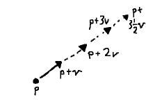
Even one vector gets us somewhere: with $ \mathbf{p} + s\mathbf{v} $, by adjusting the parameter $s$, we scale $ \mathbf{v} $ and thus move toward or away from $ \mathbf{p} $.
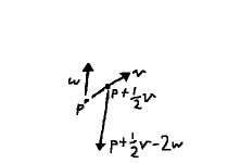
When we introduce the second parameter $t$, we add another degree of freedom. Not only are we able to move along either $ \mathbf{v} $ or $ \mathbf{w} $ relative to $ \mathbf{p} $, but we can mix them. For instance, following $ \mathbf{v} $ for half its length, then moving backward over $ \mathbf{w} $ two lengths: $ \mathbf{p} + {1 \over 2}\mathbf{v} - 2\mathbf{w} $.
In a very real way, we can think of this as being the position $ \vcomps{1 \over 2}{-2} $, with $ \mathbf{p} $ as the origin, $ \mathbf{v} $ being the x-axis, and $ \mathbf{w} $ the y-axis.
(NOTES: Comment about transformation?)
What we have is a local coordinate system, often abbreviated LCS. This is, of course, a familiar from everyday experience. We tend to speak of things from our point of view, or in terms of landmarks: "take ten steps from the big tree, then turn left". It would seem a bit of an affection to describe everything relative to the center of the universe. People would talk.
Points do have a proper location, of course. Often enough this is the more natural way to express them, as well. Static elements in a game scene, for instance, already being where they belong, stand to gain less from another point of view. Characters who run across such an element, on the other hand, might prefer them from their own perspective: in front, behind, to the right, and so on. They need to take the global coordinates and put them into local form. (TODO: image?)
The system's local origin, $ \mathbf{p} $ in the above example, would be given by something like the character's position. We want our global point, say $ \mathbf{q} $, relative to this "landmark": we are now dealing with the vector $ \mathbf{q - p} $. (TODO: image)
The parameters told us how much $ \mathbf{v} $ and $ \mathbf{w} $ were scaled, or considered differently, how far we moved along each direction. Coming at this from the other direction, we are basically wondering how similar $ \mathbf{q - p} $ is to our two vectors.
$ \mathbf{v} $ and $ \mathbf{w} $ will not always be unit vectors, so these are just the components: $ s = {\dotvwparen{v}{q - p}\over\vlen{v}} $ and $ t = {\dotvwparen{w}{q - p}\over\vlen{w}} .$ (TODO: image)
(IMAGES: 23, 24)
Right frame of mind (K)
The vectors in the foregoing example were two sides of a non-right triangle, but often they will be perpendicular unit vectors. These bring many advantages. The denominators go away in the last couple formulae, for instance, so $s$ and $t$ are a single dot product each. Furthermore, the distinction blurs between $s$ and $x$, $t$ and $y$—the sides are x- and y-axes, essentially, only shifted and reoriented.
If we do want such a coordinate system, we can often get by with one vector: thanks to the rejection and perp operator, we have ways to produce another one!
If we have three points, for instance, we might normalize the vector between two of them. Treating one of those points as the origin, we find the vector toward the third point, and then the rejection from the "line" vector to it. After normalizing this, we have what we want. (TODO: image?)
The same idea would in fact allow us to "fix" a non-perpendicular configuration: project one of the vectors onto the other, then reject from that. Normalize, et voilà! (TODO: image?)
(IMAGES: 25, 26)
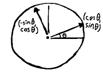
We might begin with a unit vector, on the other hand. For instance, a vector from the center of the unit circle to a point on its boundary: $ \vcomps{\cos\theta}{\sin\theta} $. The perp operator then supplies its twin: $ \vcomps{\sin\theta}{-\cos\theta} $. In fact, this actually describes a rotating coordinate system.
(NOTES: Not the conventional form... square away determinants and such)
Point-normal form (L)
(NOTES: Seems to be called the Hesse normal form)
In an earlier section we encountered the idea of a normal, a vector whose purpose is to be perpendicular to something else, typically some kind of object.
Of course, to get any use out of the normal, we need to be speaking the language of vectors. In the earlier discussion on lighting, we were only considered with how similar our two vectors were, but we might just as well focus exclusively on vectors perpendicular to the normal.
We have such a vector when its dot product with the normal is zero. Furthermore, scale them as we will, such vectors continue to point in the same or opposite direction, and thereby remain perpendicular.
On a few occasions now, we relied on the fact that between two points we find a vector. We might instead turn this around: given a vector, we assume it to mean a difference of two points, or at the very least a displacement from one.
Vectors themselves are just free-floating, having no notion of position. They acquire this once a point is brought in, as in the aforementioned cases. Adding open-ended scaling to the mix turns them into infinite lines. (TODO: image)
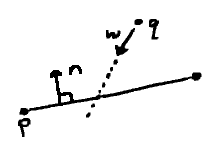
Considered as a displacement, this may be expressed as $ \mathbf{p} + t\mathbf{v} $. Here, $ \mathbf{p} $ and $ \mathbf{v} $ are a point and direction, respectively, and $t$ can be any number, ranging from zero all the way to infinity, positive or negative. This is a point-vector sum, so the result is a point. Or rather, since $t$ varies, a function that evaluates to a point. In these terms, we can express in terms of "point" $ \mathbf{x} $ as $ \mathbf{x}(t) = \mathbf{p} + t\mathbf{v}. $ At concrete values of $t$, we can ignore this function-point distinction and simply write $ \mathbf{x} $.
We know $ \dotvw{v}{n} = 0, $ from the definition of the normal. Perhaps we would get somewhere taking a dot product.
We begin with $ \dotvw{n}{x(\mathit{t})} = \dotvwparen{n}{\mathbf{p} + \textit{t}\mathbf{v}} $, then distribute the dot product on the right-hand side. One of the resulting terms vanishes, and $ \mathbf{p} $ and $ \mathbf{n} $ are both constants, so we wind up with $ \dotvw{n}{x(\mathit{t})} = c. $
This is rather strange. We have a dot product with a "point", yielding some number.
It does in fact describe a line, though. So long as the dot product of a point and the normal equals $c$, that point is on the line. (Note that $ \mathbf{p} $ is nothing special in this regard. It merely happened to be known.)
Frequently the difference-of-points form is preferred to that of displacement: $ \dotvwparen{n}{x(\mathit{t}) - p} = 0. $ This is the so-called point-normal form of a line.
As for $c$, it basically captures how far a given line comes to the origin, at its closest point. The point-normal form is essentially our earlier "which side?" formula, taking position into account. When dealing with basic vectors, which have no such notion, zero ("on the line") was a perfectly valid answer, allowing us to simply check signs. Now, we must subtract out $c$ first.
(IMAGE: 28)
Intersection: ray and line... (M)
If the point-normal form is satisfied at some $t$, $ \mathbf{x}(t) $ is a point on the line. Ordinarily, as in the previous section, we assume $ \mathbf{x}(t) $ to be roving over the line itself, and any $t$ will do.
It could just as easily be a point on a second line, say $ \mathbf{x}(t) = \mathbf{q} + t\mathbf{w}. $ We would then be seeing an intersection of two lines. Unless the lines coincide, only one value of $t$ suits this situation.
If we could find this $t$, we would be able to say "when" the lines intersected. How might we do so?
It is, of course, already right there in the point function, but everything is in vector form, whereas $t$ is a number. We need a way to extract it.
Thankfully, we have such a tool. The dot product turns vectors into numbers!
In a further instance of serendipity, the point-normal form comes equipped with one. Plugging in $ \mathbf{x}(t) $, then, we find $ \dotvwparen{n}{q + \mathit{t}w - p} = 0. $ This becomes $\dotvwparen{n}{q - p} = -t(\dotvw{n}{w}), $ and after some rearrangement: $ t = -{\dotvwparen{n}{q - p}\over\dotvw{n}{w}} $.
Since $ \mathbf{w} $ has a "forward" direction, we are really dealing with a ray, not a line. If $ t \lt 0 $, the intersection is behind $ \mathbf{q} $. We will have to decide whether this makes sense on a case-by-case basis.
If $ \mathbf{w} $ is perpendicular to $ \mathbf{n} $, we have a zero denominator above; $ \mathbf{w} $ is parallel to the line. Again we need to settle on some policies. Do we reject these situations outright, or check whether the lines are "close enough"? In any event, the intersection formula is no good to us, here; projections, distance checks, and the like become our tools of choice.
...ray and ray... (N)
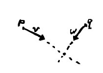
Speaking of rays, imagine how two of them, say $ \mathbf{p} + s\mathbf{v} $ and $ \mathbf{q} + t\mathbf{w} $, might intersect. (TODO: image)
Since they do so at a point, we can set the two point formulae equal: $ \mathbf{p} + s\mathbf{v} = \mathbf{q} + t\mathbf{w}. $ It then comes down to finding $s$ and $t$.
Once again we may call upon dot products to whittle our vectors down into number form. Naively doing so will only get us so far, however, since we still have two variables to solve. It would be best if we could tackle them one at a time.
$s$ and $t$ are scale factors attached to vectors. Since scale factors apply to each component, they carry through in dot products. To get rid of them, then, requires dot products of zero.
To isolate $s$, we need $t$ out of the way. This calls for a vector perpendicular to $ \mathbf{w} $. With some slight rearrangement, after applying the dot product we have $ \dotvwparen{w^{\perp}}{q - p} = s(\dotvw{w^{\perp}}{v}) $. With a little more, $ s = {\dotvwparen{w^{\perp}}{q - p}\over\dotvw{w^{\perp}}{v}}. $ Similarly, $ t = -{\dotvwparen{v^{\perp}}{q - p}\over\dotvw{v^{\perp}}{w}}. $
Once again we have to set guidelines for $ s \lt 0 $ and $ t \lt 0 $. Zero denominators have the same meaning as before, too.
Sometimes formulae like the above are expressed in terms of determinants. As we saw earlier, these soon follow when dot products and perp operators mingle.
...ray and circle (O)
Circles have gotten pretty short shrift in this discussion on vectors, but we can give them the last word as we round things out.
Recall from part 2 that a circle consists of all points a distance $r$ from a center position, say $ \mathbf{C} $. This translates quite easily to vector form. For some point $ \mathbf{x} $ on the circle we might have $ \vlen{x(\mathit{\theta}) - C} = r. $
$ \mathbf{x(\mathit{\theta})} $ is a fitting way to parametrize the circle. Following the lead of the ray-line case, however, it could just as well be a point resulting from a ray. Plugging in that same $ \mathbf{x}(t) $: $ \vlen{q + \mathit{t}w - C} = r. $
The vector length involve a square root that would be incredibly difficult to unravel. However, both sides being lengths, we can square them to get $ \vlen{q + \mathit{t}w - C}^2 = r^2. $ As mentioned earlier, a squared vector length is a dot product of the vector with itself: $ \mathbf{(q + \mathit{t}w - C)} \cdot \mathbf{(q + \mathit{t}w - C)} = r^2. $
Since the dot product distributes, we may FOIL this to obtain $ (\dotvw{w}{w})t^2 - 2(\dotvwparen{w}{q - C})t + \mathbf{(q - C)\cdot(q - C)} - r^2 = 0. $
This has the form $ at^2 + bt + c = 0, $ making it amenable to solution by the quadratic formula as $ t = {{-b \pm\sqrt{b^2 - 4ac}} \over 2a} $.
From the presence of $ t^2 $ and the ± we can deduce that there are two values of $t$. This makes sense, since the ray can enter a circle on one side and come out the other. Once again, $ t \lt 0 $ means an intersection behind $ \mathbf{q} $, which might be true for both points. If each $t$ has different sign, on the other hand, the ray only leaves the circle, meaning it must begin on the inside.
The terms inside the square root are known as the discriminant. If this is negative, the formula breaks down, giving us no solutions. This is the situation where the ray misses the circle. When it is zero, both answers are the same. This is the case of the ray grazing the circle's edge.
We only run into zero denominators when $ \dotvw{w}{w} = 0. $ We need not worry about a vector being perpendicular to itself. This only happens if $ \mathbf{w} $ is a zero vector, where our "ray" is really a point. If $ \mathbf{w} $ were a velocity, for instance, this would be an immobile object, who will obviously not be the culprit in the event of a collision. (Zero vectors can crop up in the ray-line and ray-ray cases as well, of course.)
(NOTES: Ways to simplify equation—when vector is normalized, the coefficient of 2 in $b$—, maybe mention David Eberly's stability improvements)
Summary
We now have quite an array of geometrical tools, comprising not only vectors but also insights into triangles and circles.
All this know-how is likely to wither on the vine unless we apply it. In the capstone article of this series, we will take a look at a special effect that puts many of our new-found skills to work.