
Today’s guest tutorial comes to you courtesy of X.
Intersection: ray and line... (M)
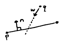
If the point-normal form is satisfied at some $t$, $ \mathbf{x}(t) $ is a point on the line. Ordinarily, as in the previous section, we assume $ \mathbf{x}(t) $ to be roving over the line itself, and any $t$ will do.
It could just as easily be a point on a second line, say $ \mathbf{x}(t) = \mathbf{q} + t\mathbf{w}. $ We would then be seeing an intersection of two lines. Unless the lines coincide, only one value of $t$ suits this situation.
If we could find this $t$, we would be able to say "when" the lines intersected. How might we do so?
It is, of course, already right there in the point function, but everything is in vector form, whereas $t$ is a number. We need a way to extract it.
Thankfully, we have such a tool. The dot product turns vectors into numbers!
In a further instance of serendipity, the point-normal form comes equipped with one. Plugging in $ \mathbf{x}(t) $, then, we find $ \dotvwparen{n}{q + \mathit{t}w - p} = 0. $ This becomes $\dotvwparen{n}{q - p} = -t(\dotvw{n}{w}), $ and after some rearrangement: $ t = -{\dotvwparen{n}{q - p}\over\dotvw{n}{w}} $.
Since $ \mathbf{w} $ has a "forward" direction, we are really dealing with a ray, not a line. If $ t \lt 0 $, the intersection is behind $ \mathbf{q} $. We will have to decide whether this makes sense on a case-by-case basis.
If $ \mathbf{w} $ is perpendicular to $ \mathbf{n} $, we have a zero denominator above; $ \mathbf{w} $ is parallel to the line. Again we need to settle on some policies. Do we reject these situations outright, or check whether the lines are "close enough"? In any event, the intersection formula is no good to us, here; projections, distance checks, and the like become our tools of choice.
...ray and ray... (N)
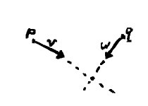
Speaking of rays, imagine how two of them, say $ \mathbf{p} + s\mathbf{v} $ and $ \mathbf{q} + t\mathbf{w} $, might intersect. (TODO: image)
Since they do so at a point, we can set the two point formulae equal: $ \mathbf{p} + s\mathbf{v} = \mathbf{q} + t\mathbf{w}. $ It then comes down to finding $s$ and $t$.
Once again we may call upon dot products to whittle our vectors down into number form. Naively doing so will only get us so far, however, since we still have two variables to solve. It would be best if we could tackle them one at a time.
$s$ and $t$ are scale factors attached to vectors. Since scale factors apply to each component, they carry through in dot products. To get rid of them, then, requires dot products of zero.
To isolate $s$, we need $t$ out of the way. This calls for a vector perpendicular to $ \mathbf{w} $. With some slight rearrangement, after applying the dot product we have $ \dotvwparen{w^{\perp}}{q - p} = s(\dotvw{w^{\perp}}{v}) $. With a little more, $ s = {\dotvwparen{w^{\perp}}{q - p}\over\dotvw{w^{\perp}}{v}}. $ Similarly, $ t = -{\dotvwparen{v^{\perp}}{q - p}\over\dotvw{v^{\perp}}{w}}. $
Once again we have to set guidelines for $ s \lt 0 $ and $ t \lt 0 $. Zero denominators have the same meaning as before, too.
Sometimes formulae like the above are expressed in terms of determinants. As we saw earlier, these soon follow when dot products and perp operators mingle.
...ray and circle (O)
Circles have gotten pretty short shrift in this discussion on vectors, but we can give them the last word as we round things out.
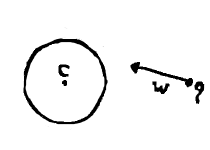
Recall from part 2 that a circle consists of all points a distance $r$ from a center position, say $ \mathbf{C} $. This translates quite easily to vector form. For some point $ \mathbf{x} $ on the circle we might have $ \vlen{x(\mathit{\theta}) - C} = r. $
$ \mathbf{x(\mathit{\theta})} $ is a fitting way to parametrize the circle. Following the lead of the ray-line case, however, it could just as well be a point resulting from a ray. Plugging in that same $ \mathbf{x}(t) $: $ \vlen{q + \mathit{t}w - C} = r. $
The vector length involve a square root that would be incredibly difficult to unravel. However, both sides being lengths, we can square them to get $ \vlen{q + \mathit{t}w - C}^2 = r^2. $ As mentioned earlier, a squared vector length is a dot product of the vector with itself: $ \mathbf{(q + \mathit{t}w - C)} \cdot \mathbf{(q + \mathit{t}w - C)} = r^2. $
Since the dot product distributes, we may FOIL this to obtain $ (\dotvw{w}{w})t^2 - 2(\dotvwparen{w}{q - C})t + \mathbf{(q - C)\cdot(q - C)} - r^2 = 0. $
This has the form $ at^2 + bt + c = 0, $ making it amenable to solution by the quadratic formula as $ t = {{-b \pm\sqrt{b^2 - 4ac}} \over 2a} $.
From the presence of $ t^2 $ and the ± we can deduce that there are two values of $t$. This makes sense, since the ray can enter a circle on one side and come out the other. Once again, $ t \lt 0 $ means an intersection behind $ \mathbf{q} $, which might be true for both points. If each $t$ has different sign, on the other hand, the ray only leaves the circle, meaning it must begin on the inside.
The terms inside the square root are known as the discriminant. If this is negative, the formula breaks down, giving us no solutions. This is the situation where the ray misses the circle. When it is zero, both answers are the same. This is the case of the ray grazing the circle's edge.
We only run into zero denominators when $ \dotvw{w}{w} = 0. $ We need not worry about a vector being perpendicular to itself. This only happens if $ \mathbf{w} $ is a zero vector, where our "ray" is really a point. If $ \mathbf{w} $ were a velocity, for instance, this would be an immobile object, who will obviously not be the culprit in the event of a collision. (Zero vectors can crop up in the ray-line and ray-ray cases as well, of course.)
(NOTES: Ways to simplify equation—when vector is normalized, the coefficient of 2 in $b$—, maybe mention David Eberly's stability improvements)
Summary
We now have quite an array of geometrical tools, comprising not only vectors but also insights into triangles and circles.
All this know-how is likely to wither on the vine unless we apply it. In the capstone article of this series, we will take a look at a special effect that puts many of our new-found skills to work.