
Today’s guest tutorial comes to you courtesy of X.
Meet the locals (J)
The $ \mathbf{p} + s\mathbf{v} + t\mathbf{w} $ construction found in the previous section is quite a powerful concept in its own right.
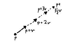
Even one vector gets us somewhere: with $ \mathbf{p} + s\mathbf{v} $, by adjusting the parameter $s$, we scale $ \mathbf{v} $ and thus move toward or away from $ \mathbf{p} $.
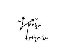
When we introduce the second parameter $t$, we add another degree of freedom. Not only are we able to move along either $ \mathbf{v} $ or $ \mathbf{w} $ relative to $ \mathbf{p} $, but we can mix them. For instance, following $ \mathbf{v} $ for half its length, then moving backward over $ \mathbf{w} $ two lengths: $ \mathbf{p} + {1 \over 2}\mathbf{v} - 2\mathbf{w} $.
In a very real way, we can think of this as being the position $ \vcomps{1 \over 2}{-2} $, with $ \mathbf{p} $ as the origin, $ \mathbf{v} $ being the x-axis, and $ \mathbf{w} $ the y-axis.
(NOTES: Comment about transformation?)
What we have is a local coordinate system, often abbreviated LCS. This is, of course, a familiar from everyday experience. We tend to speak of things from our point of view, or in terms of landmarks: "take ten steps from the big tree, then turn left". It would seem a bit of an affection to describe everything relative to the center of the universe. People would talk.
Points do have a proper location, of course. Often enough this is the more natural way to express them, as well. Static elements in a game scene, for instance, already being where they belong, stand to gain less from another point of view. Characters who run across such an element, on the other hand, might prefer them from their own perspective: in front, behind, to the right, and so on. They need to take the global coordinates and put them into local form. (TODO: image?)
The system's local origin, $ \mathbf{p} $ in the above example, would be given by something like the character's position. We want our global point, say $ \mathbf{q} $, relative to this "landmark": we are now dealing with the vector $ \mathbf{q - p} $. (TODO: image)
The parameters told us how much $ \mathbf{v} $ and $ \mathbf{w} $ were scaled, or considered differently, how far we moved along each direction. Coming at this from the other direction, we are basically wondering how similar $ \mathbf{q - p} $ is to our two vectors.
$ \mathbf{v} $ and $ \mathbf{w} $ will not always be unit vectors, so these are just the components: $ s = {\dotvwparen{v}{q - p}\over\vlen{v}} $ and $ t = {\dotvwparen{w}{q - p}\over\vlen{w}} .$ (TODO: image)
(IMAGES: 23, 24)
Right frame of mind (K)
The vectors in the foregoing example were two sides of a non-right triangle, but often they will be perpendicular unit vectors. These bring many advantages. The denominators go away in the last couple formulae, for instance, so $s$ and $t$ are a single dot product each. Furthermore, the distinction blurs between $s$ and $x$, $t$ and $y$—the sides are x- and y-axes, essentially, only shifted and reoriented.
If we do want such a coordinate system, we can often get by with one vector: thanks to the rejection and perp operator, we have ways to produce another one!
If we have three points, for instance, we might normalize the vector between two of them. Treating one of those points as the origin, we find the vector toward the third point, and then the rejection from the "line" vector to it. After normalizing this, we have what we want. (TODO: image?)
The same idea would in fact allow us to "fix" a non-perpendicular configuration: project one of the vectors onto the other, then reject from that. Normalize, et voilà! (TODO: image?)
(IMAGES: 25, 26)
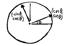
We might begin with a unit vector, on the other hand. For instance, a vector from the center of the unit circle to a point on its boundary: $ \vcomps{\cos\theta}{\sin\theta} $. The perp operator then supplies its twin: $ \vcomps{\sin\theta}{-\cos\theta} $. In fact, this actually describes a rotating coordinate system.
(NOTES: Not the conventional form... square away determinants and such)
Point-normal form (L)
(NOTES: Seems to be called the Hesse normal form)
In an earlier section we encountered the idea of a normal, a vector whose purpose is to be perpendicular to something else, typically some kind of object.
Of course, to get any use out of the normal, we need to be speaking the language of vectors. In the earlier discussion on lighting, we were only considered with how similar our two vectors were, but we might just as well focus exclusively on vectors perpendicular to the normal.
We have such a vector when its dot product with the normal is zero. Furthermore, scale them as we will, such vectors continue to point in the same or opposite direction, and thereby remain perpendicular.
On a few occasions now, we relied on the fact that between two points we find a vector. We might instead turn this around: given a vector, we assume it to mean a difference of two points, or at the very least a displacement from one.
Vectors themselves are just free-floating, having no notion of position. They acquire this once a point is brought in, as in the aforementioned cases. Adding open-ended scaling to the mix turns them into infinite lines. (TODO: image)
Considered as a displacement, this may be expressed as $ \mathbf{p} + t\mathbf{v} $. Here, $ \mathbf{p} $ and $ \mathbf{v} $ are a point and direction, respectively, and $t$ can be any number, ranging from zero all the way to infinity, positive or negative. This is a point-vector sum, so the result is a point. Or rather, since $t$ varies, a function that evaluates to a point. In these terms, we can express in terms of "point" $ \mathbf{x} $ as $ \mathbf{x}(t) = \mathbf{p} + t\mathbf{v}. $ At concrete values of $t$, we can ignore this function-point distinction and simply write $ \mathbf{x} $.
We know $ \dotvw{v}{n} = 0, $ from the definition of the normal. Perhaps we would get somewhere taking a dot product.
We begin with $ \dotvw{n}{x(\mathit{t})} = \dotvwparen{n}{\mathbf{p} + \textit{t}\mathbf{v}} $, then distribute the dot product on the right-hand side. One of the resulting terms vanishes, and $ \mathbf{p} $ and $ \mathbf{n} $ are both constants, so we wind up with $ \dotvw{n}{x(\mathit{t})} = c. $
This is rather strange. We have a dot product with a "point", yielding some number.
It does in fact describe a line, though. So long as the dot product of a point and the normal equals $c$, that point is on the line. (Note that $ \mathbf{p} $ is nothing special in this regard. It merely happened to be known.)
Frequently the difference-of-points form is preferred to that of displacement: $ \dotvwparen{n}{x(\mathit{t}) - p} = 0. $ This is the so-called point-normal form of a line.
As for $c$, it basically captures how far a given line comes to the origin, at its closest point. The point-normal form is essentially our earlier "which side?" formula, taking position into account. When dealing with basic vectors, which have no such notion, zero ("on the line") was a perfectly valid answer, allowing us to simply check signs. Now, we must subtract out $c$ first.
(IMAGE: 28)